5.7  Time Evolution Is Canonical

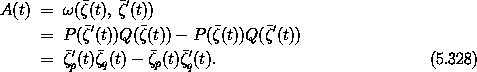
In this section we demonstrate that time evolution generates a canonical transformation: if we consider all possible initial states of a Hamiltonian system and follow all the trajectories for the same time interval, then the map from the initial state to the final state of each trajectory is a canonical transformation.

We use time evolution to generate a transformation

that is obtained in the following way. Let (t) = (t, (t), (t)) be a solution of Hamilton's equations. The transformation satisfies

or, equivalently,

Notice that changes the time component. This is the first transformation of this kind that we have considered.²⁴

Given a state (t', q', p'), we find the phase-space path emanating from this state as an initial condition, satisfying

The value (t, q, p) of (t', q', p') is then (t' + , (t' + ), (t' + )).

Time evolution is canonical if the transformation is symplectic and if the Hamiltonian transforms in an appropriate manner. The transformation is symplectic if the bilinear antisymmetric form is invariant (see equation 5.73) for a general pair of linearized state variations with zero time component.

Let ' be an increment with zero time component of the state (t', q', p'). The linearized increment in the value of (t', q', p') is = D(t', q', p') '. The image of the increment is obtained by multiplying the increment by the derivative of the transformation. On the other hand, the transformation is obtained by time evolution, so the image of the increment can also be found by the time evolution of the linearized variational system. 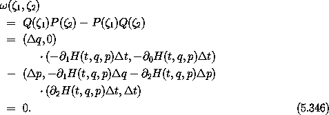Let

be variations of the state path (t) = (t, (t), (t)); then

The symplectic requirement is

This must be true for arbitrary , so it is satisfied if the following quantity is constant:

We compute the derivative:

With Hamilton's equations, the variations satisfy

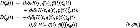
Substituting these into DA and collecting terms, we find²⁵

We conclude that time evolution generates a phase-space transformation with symplectic derivative.

To make a canonical transformation we must specify how the Hamiltonian transforms. The same Hamiltonian describes the evolution of a state and a time-advanced state because the latter is just another state. Thus the transformed Hamiltonian is the same as the original Hamiltonian.

Liouville's theorem, again

We deduced that volumes in phase space are preserved by time evolution by showing that the divergence of the phase flow is zero, using the equations of motion (see section 3.8). We can also show that volumes in phase space are preserved by the evolution using the fact that time evolution is a canonical transformation.

We have shown that phase-space volume is preserved for symplectic transformations. Now we have shown that the transformation generated by time evolution is a symplectic transformation. Therefore, the transformation generated by time evolution preserves phase-space volume. This is an alternate proof of Liouville's theorem.

Another time-evolution transformation

There is another canonical transformation that can be constructed from time evolution. We define the transformation ' such that

where S(a, b, c) = (a + , b, c) shifts the time of a phase-space state.²⁶ More explicitly, given a state (t, q', p'), we evolve the state that is obtained by subtracting from t; that is, we take the state (t - , q', p') as an initial state for evolution by Hamilton's equations. The state path satisfies

The output of the transformation is the state

The transformation satisfies

The arguments of ' are not a consistent phase-space state; the time argument must be decremented by to obtain a consistent state. The transformation is completed by evolution of this consistent state.

Why is this a good idea? Our usual canonical transformations do not change the time component. This modified time-evolution transformation is thus of the form discussed previously. The resulting time-evolution transformation is canonical and in the usual form:

This transformation can also be extended to be a canonical transformation, with an appropriate adjustment of the Hamiltonian. The Hamiltonian H' that gives the correct Hamilton's equations at the transformed phase-space point is the original Hamiltonian composed with a function that decrements the independent variable by :

or

Notice that if H is time independent then H' = H.

Assume we have a procedure C such that ((C delta-t) state) implements a time-evolution transformation of the state state with time interval delta-t; then the procedure Cp such that ((Cp delta-t) state) implements ' of the same state and time interval can be derived from the procedure C by using the procedure

(define ((C->Cp C) delta-t)
  (compose (C delta-t) (shift-t (- delta-t))))

where shift-t implements S:

(define ((shift-t delta-t) state)
  (up 
   (+ (time state) delta-t)
   (coordinate state)
   (momentum state)))

To complete the canonical transformation we have a procedure that transforms the Hamiltonian:

(define ((H->Hp delta-t) H)
  (compose H (shift-t (- delta-t))))

So both and ' can be used to make canonical transformations by specifying how the old and new Hamiltonians are related. For the Hamiltonian is unchanged. For ' the Hamiltonian is time shifted.

Exercise 5.21.  Verification
The condition (5.19) that Hamilton's equations are preserved for is

and the condition that Hamilton's equations are preserved for ' is

Verify that these conditions are satisfied.

Exercise 5.22.  Driven harmonic oscillator
We can use the simple driven harmonic oscillator to illustrate that time evolution yields a symplectic transformation that can be extended to be canonical in two ways. We use the driven harmonic oscillator because its solution can be compactly expressed in explicit form.

Suppose that we have a harmonic oscillator with natural frequency ₀ driven by a periodic sinusoidal drive of frequency and amplitude . The Hamiltonian we will consider is

The general solution for a given initial state (t₀, q₀, p₀) evolved for a time is

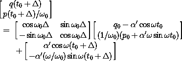
where ' = /(₀² - ²).

a.  Fill in the details of the procedure

(define (((C alpha omega omega0) delta-t) state)
   ... )

that implements the time-evolution transformation of the driven harmonic oscillator.

b.  In terms of C, the general solution emanating from a given state is

(define (((solution alpha omega omega0) state0) t)
  (((C alpha omega omega0) (- t (time state0))) state0))

Check that the implementation of C is correct by using it to construct the solution and verifying that the solution satisfies Hamilton's equations. Further check the solution by comparing to numerical integration.

c.  We know that for any phase-space state function F the rate of change of that function along a solution path is

Show, by writing a short program to test it, that this is true of the function implemented by (C delta) for the driven oscillator. Why is this interesting?

d.  Verify that both C and Cp are symplectic using symplectic?.

e.  Use the procedure canonical? to verify that both C and Cp are canonical with the appropriate transformed Hamiltonian.

5.7.1  Another View of Time Evolution

We can also show that time evolution generates canonical transformations using the Poincaré-Cartan integral invariant.

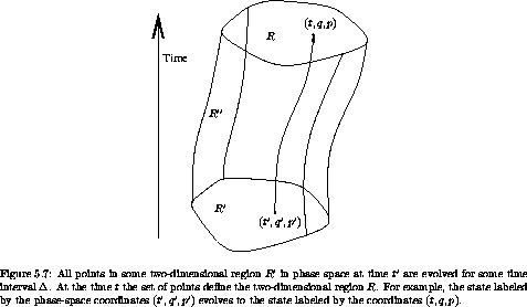
Consider a two-dimensional region of phase-space coordinates, R', at some particular time t' (see figure 5.8). Let R be the image of this region at time t under time evolution for a time interval of . The time evolution is governed by a Hamiltonian H. Let sum_i A_i be the sum of the oriented areas of the projections of R onto the fundamental canonical planes.²⁷ Similarly, let sum_i A'_i be the sum of oriented projected areas for R'. We will show that sum_i A_i = sum_i A'_i, and thus the Poincaré integral invariant is preserved by time evolution. By showing that the Poincaré integral invariant is preserved, we will have shown that the qp part of the transformation generated by time evolution is symplectic. From this we can construct canonical transformations from time evolution as before.

In the extended phase space we see that the evolution sweeps out a cylindrical volume with endcaps R' and R, each at a fixed time. Let R'' be the two-dimensional region swept out by the trajectories that map the boundary of region R' to the boundary of region R. The regions R, R', and R'' together form the boundary of a volume of phase-state space.

The Poincaré-Cartan integral invariant on the whole boundary is zero.²⁸ Thus

where the n index indicates the t, p_t canonical plane. The second term is negative, because in the extended phase space we take the area to be positive if the normal to the surface is outward pointing.

We will show that the Poincaré-Cartan integral invariant for a region of phase space that is generated by time evolution is zero:

This will allow us to conclude

The areas of the projection of R and R' on the t, p_t plane are zero because R and R' are at constant times, so for these regions the Poincaré-Cartan integral invariant is the same as the Poincaré integral invariant. Thus

We are left with showing that the Poincaré-Cartan integral invariant for the region R'' is zero. This will be zero if the contribution from any small piece of R'' is zero. We will show this by showing that the form (see equation 5.71) on a small parallelogram in this region is zero. Let (0; q, t; p, p_t) be a vertex of this parallelogram. The parallelogram is specified by two edges ₁ and ₂ emanating from this vertex with components (0; q, t; p, p_t). For edge ₁ of the parallelogram, we take a constant-time phase-space increment with length q and p in the q and p directions. The first-order change in the Hamiltonian that corresponds to these changes is

for constant time t = 0. The increment p_t is the negative of H. So the extended phase-space increment is

The edge ₂ is obtained by time evolution of the vertex for a time interval t. Using Hamilton's equations, we obtain

The form applied to these incremental states that form the edges of this parallelogram gives the area of the parallelogram:

So we may conclude that the integral of this expression over the entire surface of the tube of trajectories is also zero. Thus the Poincaré-Cartan integral invariant is zero for any region that is generated by time evolution.

Having proven that the trajectory tube provides no contribution, we have shown that the Poincaré integral invariant of the two endcaps is the same. This proves that time evolution generates a symplectic qp transformation.

Area preservation of surfaces of section

We can use the Poincaré-Cartan invariant to prove that for autonomous two-degree-of-freedom systems surfaces of section (constructed appropriately) preserve area.

To show this we consider a surface of section for one coordinate (say q₂) equal to zero. We construct the section by accumulating the (q₁, p₁) pairs. We assume that all initial conditions have the same energy. We compute the sum of the areas of canonical projections in the extended phase space again. Because all initial conditions have the same q₂ = 0 there is no area on the q₂, p₂ plane, and because all the trajectories have the same value of the Hamiltonian the area of the projection on the t, p_t plane is also zero. So the sum of areas of the projections is just the area of the region on the surface of section. Now let each point on the surface of section evolve to the next section crossing. For each point on the section this may take a different amount of time. Compute the sum of the areas again for the mapped region. Again, all points of the mapped region have the same q₂ so the area on the q₂, p₂ plane is zero, and they continue to have the same energy so the area on the t, p_t plane is zero. So the area of the mapped region is again just the area on the surface of section, the q₁, p₁ plane. Time evolution preserves the sum of areas, so the area on the surface of section is the same as the mapped area.

So surfaces of section preserve area provided that the section points are entirely on a canonical plane. For example, to make the Hénon-Heiles surfaces of section (see section 3.6.3) we plotted p_y versus y when x = 0 with p_x > 0. So for all section points the x coordinate has the fixed value 0, the trajectories all have the same energy, and the points accumulated are entirely in the y, p_y canonical plane. So the Hénon-Heiles surfaces of section preserve area.

5.7.2  Yet Another View of Time Evolution

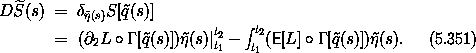
We can show that time evolution generates a symplectic transformation directly from the action principle.

Recall that the Lagrangian action S is

We computed the variation of the action in deriving the Lagrange equations. The variation is (see equation 1.33)

rewritten in terms of the Euler-Lagrange operator E. In the derivation of the Lagrange equations we considered only variations that preserved the endpoints of the path being tested. However, equation (5.347) is true of arbitrary variations. Here we consider variations that are not zero at the endpoints around a realizable path q (one for which E [ L ] o [q] = 0 ). For these variations the variation of the action is just the integrated term:

Recall that p and are structures, and the product implies a sum of products of components.

Consider a continuous family of realizable paths; the path for parameter s is (s) and the coordinates of this path at time t are (s)(t). We define (s) = D(s); the variation of the path along the family is the derivative of the parametric path with respect to the parameter. Let

be the value of the action from t₁ to t₂ for path (s). The derivative of the action along this parametric family of paths is²⁹

Because (s) is a realizable path, E[L] o [(s)] = 0. So

where (s) is the conjugate momentum to (s). The integral of D is

where

In conventional notation the latter line integral is written

where ₁(s) = (s)(t₁) and ₂(s) = (s)(t₂).

For a loop family of paths (such that (s₂) = (s₁)), the difference of actions at the endpoints vanishes, so we deduce

which is the line-integral version of the integral invariants.

In terms of area integrals, using Stokes's theorem, this is

where Rⁱ_j are the regions in the ith canonical plane. We have found that the time evolution preserves the integral invariants, and thus time evolution generates a symplectic transformation.