
The principle of stationary action characterizes the realizable paths of systems in configuration space as those for which the action has a stationary value. In elementary calculus, we learn that the critical points of a function are the points where the derivative vanishes. In an analogous way, the paths along which the action is stationary are solutions of a system of differential equations. This system, called the Euler-Lagrange equations or just the Lagrange equations, is the link that permits us to use the principle of stationary action to compute the motions of mechanical systems, and to relate the variational and Newtonian formulations of mechanics.48
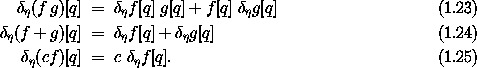
We will find that if L is a Lagrangian for a system that depends on time, coordinates, and velocities, and if q is a coordinate path for which the action S[q](t1, t2) is stationary (with respect to any variation in the path that keeps the endpoints of the path fixed), then
Here L is a real-valued function of a local tuple;
 1 L and 2 L denote the partial derivatives
of L with respect to its generalized position and generalized
velocity arguments.49
The function 2 L maps a local tuple to a structure
whose components are the
derivatives of L with respect to each component of the generalized velocity.
The function
1 L and 2 L denote the partial derivatives
of L with respect to its generalized position and generalized
velocity arguments.49
The function 2 L maps a local tuple to a structure
whose components are the
derivatives of L with respect to each component of the generalized velocity.
The function  [q] maps time to the local tuple:
[q](t) = ( t, q(t), Dq(t), ... ).
Thus the compositions 1 L o
[q] and 2 L o [q] are functions of one argument,
time. The Lagrange equations assert that the derivative of 2
L o [q] is equal to 1 L
o [q], at any time.
Given a Lagrangian,
the Lagrange equations form a system of ordinary differential equations
that must be satisfied by realizable paths.50
[q] maps time to the local tuple:
[q](t) = ( t, q(t), Dq(t), ... ).
Thus the compositions 1 L o
[q] and 2 L o [q] are functions of one argument,
time. The Lagrange equations assert that the derivative of 2
L o [q] is equal to 1 L
o [q], at any time.
Given a Lagrangian,
the Lagrange equations form a system of ordinary differential equations
that must be satisfied by realizable paths.50
We will show that principle of stationary action implies that realizable paths satisfy a set of ordinary differential equations. First we will develop tools for investigating how path-dependent functions vary as the paths are varied. We will then apply these tools to the action, to derive the Lagrange equations.
Suppose that we have a function f[q] that depends on a path q.
How does the function vary as the path is varied? Let q be a
coordinate path and q + 
 be a varied path, where the function
is a path-like function that can be added to the path q, and the
factor is a scale factor. We define the variation
be a varied path, where the function
is a path-like function that can be added to the path q, and the
factor is a scale factor. We define the variation
 f[q] of the function f on the path q by51

The variation of f is a linear approximation to the change in the
function f for small variations in the path. The variation of f
depends on .
A simple example is the variation of the identity path function: I[q] = q. Applying the definition, we find

It is traditional to write I[q] simply as q.
Another example is the variation of the path function that returns
the derivative of the path. We have

It is traditional to write g[q] as Dq.
The variation may be represented in terms of a derivative. Let g()
= f[q + ]; then

Variations have the following derivative-like properties. For path-dependent functions f and g and constant c:
Let F be a path-independent function and g be a path-dependent function; then

The operators D (differentiation) and (variation)
commute in the following sense:

Variations also commute with integration in a similar sense.
If a path-dependent function f is stationary for a particular path
q with respect to small changes in that path, then it must be
stationary for a subset of those variations that results from adding
small multiples of a particular function to q. So the
statement f[q] = 0 for arbitrary implies the
function f is stationary for small variations of the path around q.
Exercise 1.7. Properties of
Show that has the
properties 1.23-1.27.
Exercise 1.8. Implementation of
a. Suppose we have a procedure f that implements a path-dependent
function: for path q and time t it has the value
((f q) t).
The procedure delta computes the
variation ( f)[q](t) as the value of the expression ((((delta eta)
f) q) t).
Complete the definition of delta:
(define (((delta eta) f) q)
... )
b. Use your delta procedure to verify the properties of
listed in exercise 1.7 for simple functions
such as implemented by the procedure f:
(define (f q)
(compose
(literal-function 'F (-> (UP Real Real Real) Real))
(Gamma q)))
This implements a one-degree-of-freedom path-dependent function that depends on the local tuple of the path at each moment. You should compute both sides of the equalities and compare the results.
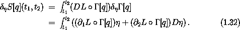
The action is the integral of the Lagrangian along a path:

For a realizable path q the variation of the action with respect to
any variation that preserves the endpoints, (t1) =
(t2) = 0, is zero:

Variation commutes with integration, so the variation of the action is


which follows from equations (1.20) and (1.21), and using the chain rule for variations (1.26), we get52
Integrating the last term of equation (1.32) by parts gives
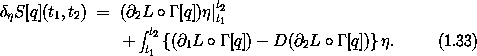
For our variation we have (t1) = (t2) = 0, so
the first term vanishes.
Thus the variation of the action is zero if and only if

The variation of the action is zero because, by assumption, q is a
realizable path.
Thus (1.34) must be true for any
function that is zero at the endpoints.
We retain enough freedom in the choice of the variation that
the factor in the integrand multiplying is forced to be zero at
each point along the path. We argue by contradiction: Suppose this
factor were nonzero at some particular time. Then it would have to be
nonzero in at least one of its components. But if we choose our
to be a bump that is nonzero only in that component in a
neighborhood of that time, and zero everywhere else, then the integral
will be nonzero.
So we may conclude that the factor in curly brackets is identically zero:53

This is just what we set out to obtain, the Lagrange equations.
A path satisfying Lagrange's equations is one for which the action is stationary, and the fact that the action is stationary depends only on the values of L at each point of the path (and at each point on nearby paths), not on the coordinate system we use to compute these values. So if the system's path satisfies Lagrange's equations in some particular coordinate system, it must satisfy Lagrange's equations in any coordinate system. Thus the equations of variational mechanics are derived the same way in any configuration space and any coordinate system.
For an example, consider the harmonic oscillator. A Lagrangian is


The Lagrangian is applied to a tuple of the time, a coordinate, and a velocity. The symbols t, x, and v are arbitrary; they are used to specify formal parameters of the Lagrangian.
Now suppose we have a configuration path y, which gives the coordinate of the oscillator y(t) for each time t. The initial segment of the corresponding local tuple at time t is


which is the equation of motion of the harmonic oscillator.
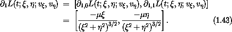
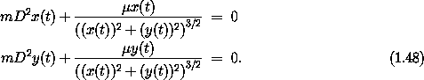
As another example, consider the two-dimensional motion of a particle of mass m with gravitational potential energy - µ/r, where r is the distance to the center of attraction. A Lagrangian is54

where  and are formal parameters for rectangular
coordinates of the particle, and v and v are formal
parameters for corresponding rectangular velocity components. Then55
and are formal parameters for rectangular
coordinates of the particle, and v and v are formal
parameters for corresponding rectangular velocity components. Then55

Now suppose we have a configuration path q = ( x, y ), so that the coordinate tuple at time t is q(t) = ( x(t), y(t) ). The initial segment of the local tuple at time t is

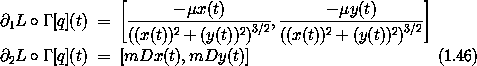

The component Lagrange equations at time t are
Exercise 1.9. Lagrange's equations
Derive the Lagrange equations for the following systems, showing
all of the intermediate steps as in the harmonic oscillator and
orbital motion examples.
a. A particle of mass m moves in a two-dimensional potential V(x, y) = (x2 + y2)/2 + x2 y - y3/3, where x and y are rectangular coordinates of the particle. A Lagrangian is L(t; x, y; vx, vy) = (1/2) m (vx2 + vy2) - V(x, y).
b. An ideal planar pendulum consists of a bob of mass m connected
to a pivot by a massless rod of length l subject to uniform
gravitational acceleration g. A Lagrangian is L(t,  ,
,
 ) = (1/2) m l2 2 + m g l cos .
The formal parameters of L are t,
, and ; measures the
angle of the pendulum rod to a plumb line and is the
angular velocity of the rod.56
) = (1/2) m l2 2 + m g l cos .
The formal parameters of L are t,
, and ; measures the
angle of the pendulum rod to a plumb line and is the
angular velocity of the rod.56
c. A Lagrangian for a particle of mass m constrained to move
on a sphere of radius R is L(t; ,  ;
;  , ß) =
(1/2) m R2 (2 + (ß sin )2). The angle
is the colatitude of the particle and is the longitude; the rate of
change of the colatitude is and the rate of change of the
longitude is ß.
, ß) =
(1/2) m R2 (2 + (ß sin )2). The angle
is the colatitude of the particle and is the longitude; the rate of
change of the colatitude is and the rate of change of the
longitude is ß.
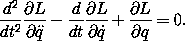
Exercise 1.10. Higher-derivative Lagrangians
Derive Lagrange's equations for Lagrangians that depend on
accelerations. In particular, show that the Lagrange equations for Lagrangians of the form
L(t, q,  ,
,  ) with terms are57

In general, these equations, first derived by Poisson, will involve the fourth derivative of q. Note that the derivation is completely analogous to the derivation of the Lagrange equations without accelerations; it is just longer. What restrictions must we place on the variations so that the critical path satisfies a differential equation?
The procedure for
computing Lagrange's equations mirrors the functional
expression (1.18), where the procedure Gamma implements :58
(define ((Lagrange-equations Lagrangian) q)
(- (D (compose ((partial 2) Lagrangian) (Gamma q)))
(compose ((partial 1) Lagrangian) (Gamma q))))
The argument of Lagrange-equations is a procedure that computes a Lagrangian. It returns a procedure that when applied to a path q returns a procedure of one argument (time) that computes the left-hand side of the Lagrange equations (1.18). These residual values are zero if q is a path for which the Lagrangian action is stationary.
Observe that the Lagrange-equations procedure, like the Lagrange equations themselves, is valid for any generalized coordinate system. When we write programs to investigate particular systems, the procedures that implement the Lagrangian function and the path q will reflect the actual coordinates chosen to represent the system, but we use the same Lagrange-equations procedure in each case. This abstraction reflects the important fact that the method of derivation of Lagrange's equations from a Lagrangian is always the same; it is independent of the number of degrees of freedom, the topology of the configuration space, and the coordinate system used to describe points in the configuration space.
Consider again the case of a free particle. The Lagrangian is
implemented by the procedure L-free-particle. Rather
than numerically integrating and minimizing the action, as we did
in section 1.4, we can check Lagrange's equations for an arbitrary
straight-line path t  ( at + a0, bt + b0, ct + c0 ):
(define (test-path t)
(up (+ (* 'a t) 'a0)
(+ (* 'b t) 'b0)
(+ (* 'c t) 'c0)))
(print-expression
(((Lagrange-equations (L-free-particle 'm))
test-path)
't))
(down 0 0 0)
That the residuals are zero indicates that the test path satisfies the Lagrange equations.59
We can also apply the Lagrange-equations procedure to an arbitrary function:60
(show-expression
(((Lagrange-equations (L-free-particle 'm))
(literal-function 'x))
't))
(* (((expt D 2) x) t) m)

The result is an expression containing the arbitrary time t and mass m, so it is zero precisely when D2 x = 0, which is the expected equation for a free particle.
Consider the harmonic oscillator again, with Lagrangian (1.16). We know that the motion of a harmonic oscillator is a sinusoid with a given amplitude, frequency, and phase:

Suppose we have forgotten how the constants in the solution relate to the physical parameters of the oscillator. Let's plug in the proposed solution and look at the residual:
(define (proposed-solution t)
(* 'a (cos (+ (* 'omega t) 'phi))))
(show-expression
(((Lagrange-equations (L-harmonic 'm 'k))
proposed-solution)
't))
The residual here shows that for nonzero amplitude, the only solutions
allowed are ones where ( k - m  2 ) = 0 or
= (k/m)1/2.
2 ) = 0 or
= (k/m)1/2.
Exercise 1.11.
Compute Lagrange's equations for the Lagrangians in
exercise 1.9 using the Lagrange-equations procedure. Additionally, use the computer to
perform each of the steps in the Lagrange-equations procedure
and show the intermediate results. Relate these steps to the ones you
showed in the hand derivation of exercise 1.9.
Exercise 1.12.
a. Write a procedure to compute the Lagrange equations for
Lagrangians that depend upon acceleration, as in
exercise 1.10. Note that Gamma can take an optional argument giving
the length of the initial segment
of the local tuple needed. The default length is 3, giving
components of the local tuple up to and including the velocities.
b. Use your procedure to compute the Lagrange equations for the Lagrangian

Do you recognize the resulting equation of motion?
c. For more fun, write the general Lagrange equation procedure that takes a Lagrangian of any order, and the order, to produce the required equations of motion.
48 This result was initially discovered by Euler and later rederived by Lagrange.
49 The derivative or partial derivative of a function that takes structured arguments is a new function that takes the same number and type of arguments. The range of this new function is itself a structure with the same number of components as the argument with respect to which the function is differentiated.
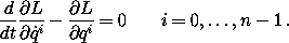
50 Lagrange's equations are traditionally written in the form
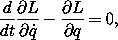
or, if we write a separate equation for each component of q, as
In this way of writing Lagrange's equations the notation
does not distinguish between L, which is a real-valued function of
three variables (t, q, ), and L o [q], which is
a real-valued function of one real variable t. If we do not
realize this notational pun, the equations don't make sense as
written -- L/ is a function of three
variables, so we must regard the arguments q, as functions
of t before taking d/dt of the expression. Similarly,
L/ q is a function of three variables, which we must view
as a function of t before setting it equal to d/dt(
L/ ). These implicit applications of the chain
rule pose no problem in performing hand computations -- once you
understand what the equations represent.
51 The variation operator is like the derivative operator in
that it acts on the immediately following function: f[q] =
( f)[q].
52 A function of multiple arguments is considered a function of a tuple of its arguments. Thus, the derivative of a function of multiple arguments is a tuple of the partial derivatives of that function with respect to each of the arguments. So in the case of a Lagrangian L,

53 To make this argument more precise requires careful analysis.
54 When we write a definition that names the components of the local tuple, we indicate that these are grouped into time, position, and velocity components by separating the groups with semicolons.
55 The derivative with respect to a tuple is a tuple of the partial derivatives with respect to each component of the tuple (see the appendix on notation).
56 The symbol is just a mnemonic symbol; the dot
over the does not indicate differentiation. To
define L we could have just as well have written: L(a, b, c) = (1/2) m
l2 c2 + m g l cos b. However, we use a dotted symbol to remind us
that the argument matching a formal parameter, such as ,
is a rate of change of an angle, such as .
57 In traditional notation these equations read
58 The Lagrange-equations procedure uses the operations (partial 1) and (partial 2), which implement the partial derivative operators with respect to the second and third argument positions (those with indices 1 and 2).
59 There is a Lagrange equation for every degree of freedom. The residuals of all the equations are zero if the path is realizable. The residuals are arranged in a down tuple because they result from derivatives of the Lagrangian with respect to argument slots that take up tuples. See the appendix on notation.
60 Observe that the second derivative is indicated as the square of the derivative operator (expt D 2). Arithmetic operations in Scmutils extend over operators as well as functions.