 is (1/2) m v2, where v is the
magnitude of . In this case we can choose the generalized
coordinates to be the ordinary rectangular coordinates.
is (1/2) m v2, where v is the
magnitude of . In this case we can choose the generalized
coordinates to be the ordinary rectangular coordinates.
To illustrate the above ideas, and to introduce their formulation as
computer programs, we consider the simplest mechanical system -- a
free particle moving in three dimensions. Euler and Lagrange discovered that for
a free particle the time integral of the kinetic energy over the
particle's actual path is smaller than the same integral along any
alternative path between the same points: a free particle moves
according to the principle of stationary action, provided we take the
Lagrangian to be the kinetic energy. The kinetic energy for a particle of
mass m and velocity is (1/2) m v2, where v is the
magnitude of . In this case we can choose the generalized
coordinates to be the ordinary rectangular coordinates.
Following Euler and Lagrange, the Lagrangian for the free particle is26

where the formal parameter x names a tuple of components of the position with respect to a given rectangular coordinate system, and the formal parameter v names a tuple of velocity components.27
We can express this formula as a procedure:
(define ((L-free-particle mass) local)
(let ((v (velocity local)))
(* 1/2 mass (dot-product v v))))
The definition indicates that L-free-particle is a procedure that takes mass as an argument and returns a procedure that takes a local tuple local,28 extracts the generalized velocity with the procedure velocity, and uses the velocity to compute the value of the Lagrangian.
Suppose we let q denote a coordinate path function that maps time to position components:29

We can make this definition30
(define q
(up (literal-function 'x)
(literal-function 'y)
(literal-function 'z)))
where literal-function makes a procedure that represents a function of one argument that has no known properties other than the given symbolic name. The symbol q now names a procedure of one real argument (time) that produces a tuple of three components representing the coordinates at that time. For example, we can evaluate this procedure for a symbolic time t as follows:
(print-expression (q 't))
(up (x t) (y t) (z t))
The procedure print-expression produces a printable form of the expression, and simplifies expressions before printing them.
The derivative of the coordinate path Dq is the function that maps time to velocity components:

We can make and use the derivative of a function.31 For example, we can write:
(print-expression ((D q) 't))
(up ((D x) t) ((D y) t) ((D z) t))
The function  takes a coordinate path and returns a function
of time that gives the local tuple ( t, q(t), Dq(t), ... ).
We implement this with the procedure Gamma. Here is
what Gamma does:
takes a coordinate path and returns a function
of time that gives the local tuple ( t, q(t), Dq(t), ... ).
We implement this with the procedure Gamma. Here is
what Gamma does:
(print-expression ((Gamma q) 't))
(up t
(up (x t) (y t) (z t))
(up ((D x) t) ((D y) t) ((D z) t)))
So the composition L o is a function of time that returns the
value of the Lagrangian for this point on the path:32
(print-expression
((compose (L-free-particle 'm) (Gamma q)) 't))
(+ (* 1/2 m (expt ((D x) t) 2))
(* 1/2 m (expt ((D y) t) 2))
(* 1/2 m (expt ((D z) t) 2)))
The procedure show-expression is like print-expression except that it puts the simplified expression into traditional infix form and displays the result.33 We use this method of display to make the boxed expressions in this book. The procedure show-expression also produces the prefix form as returned by print-expression, but we usually do not show this.34
(show-expression
((compose (L-free-particle 'm) (Gamma q)) 't))
According to equation (1.11) we can compute the Lagrangian action from time t1 to time t2 as:
(define (Lagrangian-action L q t1 t2)
(definite-integral (compose L (Gamma q)) t1 t2))
Lagrangian-action takes as arguments a procedure L that computes the Lagrangian, a procedure q that computes a coordinate path, and starting and ending times t1 and t2. The definiteintegral used here takes as arguments a function and two limits t1 and t2, and computes the definite integral of the function over the interval from t1 to t2.35 Notice that the definition of Lagrangian-action does not depend on any particular set of coordinates or even the dimension of the configuration space. The method of computing the action from the coordinate representation of a Lagrangian and a coordinate path does not depend on the coordinate system.
We can now compute the action for the free particle along a path. For
example, consider a particle moving at uniform speed along a straight
line t  ( 4t + 7, 3t + 5, 2t + 1 ).36 We represent
the path as a procedure
( 4t + 7, 3t + 5, 2t + 1 ).36 We represent
the path as a procedure
(define (test-path t)
(up (+ (* 4 t) 7)
(+ (* 3 t) 5)
(+ (* 2 t) 1)))
For a particle of mass 3, we obtain the action between t = 0 and t = 10 as37
(Lagrangian-action (L-free-particle 3.0) test-path 0.0 10.0)
435.
Exercise 1.4. Lagrangian actions
For a free particle an appropriate Lagrangian is38
Suppose that x is the constant-velocity straight-line path of a free particle, such that xa = x(ta) and xb = x(tb). Show that the action on the solution path is

We already know that the actual path of a free particle is
uniform motion in a straight line. According to Euler and
Lagrange, the action is smaller along a straight-line test
path than along nearby paths. Let q be a
straight-line test path with action S[q](t1, t2). Let q +

 be a
nearby path, obtained from q by adding a path variation
scaled by the real parameter .39
The action on the varied path is
S[q + ](t1, t2). Euler and Lagrange found that S[q +
](t1, t2) > S[q](t1, t2) for any that is zero at the
endpoints and for any small nonzero .
be a
nearby path, obtained from q by adding a path variation
scaled by the real parameter .39
The action on the varied path is
S[q + ](t1, t2). Euler and Lagrange found that S[q +
](t1, t2) > S[q](t1, t2) for any that is zero at the
endpoints and for any small nonzero .
Let's check this numerically by varying the test path, adding some
amount of a test function that is zero at the endpoints t = t1 and
t = t2. To make a function that is zero at the endpoints,
given a sufficiently well-behaved function  , we can use
(t) = (t - t1)(t - t2)(t). This can be implemented:
, we can use
(t) = (t - t1)(t - t2)(t). This can be implemented:
(define ((make-eta nu t1 t2) t)
(* (- t t1) (- t t2) (nu t)))
We can use this to compute the action for a free particle over
a path varied from the given path, as a function of :40
(define ((varied-free-particle-action mass q nu t1 t2) epsilon)
(let ((eta (make-eta nu t1 t2)))
(Lagrangian-action (L-free-particle mass)
(+ q (* epsilon eta))
t1
t2)))
The action for the varied path, with (t) = ( sin t, cos t,
t2 )
and = 0.001, is, as expected, larger than for the test path:
((varied-free-particle-action 3.0 test-path
(up sin cos square)
0.0 10.0)
0.001)
436.29121428571153
We can numerically compute the value of for which the action is
minimized. We search between, say, - 2 and 1:41
(minimize
(varied-free-particle-action 3.0 test-path
(up sin cos square)
0.0 10.0)
-2.0 1.0)
(-1.5987211554602254e-14 435.0000000000237 5)
We find exactly what is expected -- that the best value for is
zero,42
and the minimum value of the action is the action along the
straight path.
We have used the variational principle to determine if a given trajectory is realizable. We can also use the variational principle to find trajectories. Given a set of trajectories that are specified by a finite number of parameters, we can search the parameter space looking for the trajectory in the set that best approximates the real trajectory by finding one that minimizes the action. By choosing a good set of approximating functions we can get arbitrarily close to the real trajectory.43
One way to make a parametric path that has fixed endpoints is to use a polynomial that goes through the endpoints as well as a number of intermediate points. Variation of the positions of the intermediate points varies the path; the parameters of the varied path are the coordinates of the intermediate positions. The procedure make-path constructs such a path using a Lagrange interpolation polynomial.44 The procedure make-path is called with five arguments: (make-path t0 q0 t1 q1 qs), where q0 and q1 are the endpoints, t0 and t1 are the corresponding times, and qs is a list of intermediate points.
Having specified a parametric path, we can construct a parametric action that is just the action computed along the parametric path:
(define ((parametric-path-action Lagrangian t0 q0 t1 q1) qs)
(let ((path (make-path t0 q0 t1 q1 qs)))
(Lagrangian-action Lagrangian path t0 t1)))
We can find approximate solution paths by finding parameters that minimize the action. We do this minimization with a canned multidimensional minimization procedure:45
(define (find-path Lagrangian t0 q0 t1 q1 n)
(let ((initial-qs (linear-interpolants q0 q1 n)))
(let ((minimizing-qs
(multidimensional-minimize
(parametric-path-action Lagrangian t0 q0 t1 q1)
initial-qs)))
(make-path t0 q0 t1 q1 minimizing-qs))))
The procedure multidimensional-minimize takes a procedure (in this case the value of the call to parametricpathaction) that computes the function to be minimized (in this case the action) and an initial guess for the parameters. Here we choose the initial guess to be equally spaced points on a straight line between the two endpoints, computed with linear-interpolants.
To illustrate the use of this strategy, we will find trajectories of the harmonic oscillator, with Lagrangian46

for mass m and spring constant k. This Lagrangian is implemented by
(define ((L-harmonic m k) local)
(let ((q (coordinate local))
(v (velocity local)))
(- (* 1/2 m (square v)) (* 1/2 k (square q)))))
We can find an approximate path taken by the harmonic oscillator for
m = 1 and k = 1 between q(0) = 1 and q( /2) = 0 as follows:47
(define q (find-path (L-harmonic 1.0 1.0) 0. 1. :pi/2 0. 3))
We know that the trajectories of this harmonic oscillator, for m = 1 and k = 1, are

where the amplitude A and the phase  are determined by the
initial conditions. For the chosen endpoint conditions the solution
is q(t) = cos(t). The approximate path should be an approximation to
cosine over the range from 0 to /2.
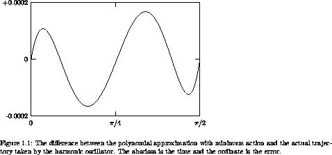
Figure 1.1 shows the error in the polynomial
approximation produced by this process. The maximum error in the
approximation with three intermediate points is less than 1.7×
10-4. We find, as expected, that the error in the approximation
decreases as the number of intermediate points is increased. For four
intermediate points it is about a factor of 15 better.
are determined by the
initial conditions. For the chosen endpoint conditions the solution
is q(t) = cos(t). The approximate path should be an approximation to
cosine over the range from 0 to /2.
Figure 1.1 shows the error in the polynomial
approximation produced by this process. The maximum error in the
approximation with three intermediate points is less than 1.7×
10-4. We find, as expected, that the error in the approximation
decreases as the number of intermediate points is increased. For four
intermediate points it is about a factor of 15 better.
Exercise 1.5. Solution process
We can watch the progress of the minimization by modifying the
procedure parametric-path-action to plot the path
each time the action is computed. Try this:
(define win2 (frame 0. :pi/2 0. 1.2))
(define ((parametric-path-action Lagrangian t0 q0 t1 q1)
intermediate-qs)
(let ((path (make-path t0 q0 t1 q1 intermediate-qs)))
;; display path
(graphics-clear win2)
(plot-function win2 path t0 t1 (/ (- t1 t0) 100))
;; compute action
(Lagrangian-action Lagrangian path t0 t1)))
(find-path (L-harmonic 1. 1.) 0. 1. :pi/2 0. 2)
Exercise 1.6. Minimizing action
Suppose we try to obtain a path by minimizing an action for an
impossible problem. For example, suppose we have a free particle and
we impose endpoint conditions on the velocities as well as the
positions that are inconsistent with the particle being free. Does
the formalism protect itself from such an unpleasant attack? You may find
it illuminating to program it and see what happens.
26 Here we are making a function definition. A definition specifies the value of the function for arbitrarily chosen formal parameters. One may change the name of a formal parameter, so long as the new name does not conflict with any other symbol in the definition. For example, the following definition specifies exactly the same free-particle Lagrangian:
27 The Lagrangian is formally a function of the local tuple, but any particular Lagrangian depends only on a finite initial segment of the local tuple. We define functions of local tuples by explicitly declaring names for the elements of the initial segment of the local tuple that includes the elements upon which the function depends.
28 We represent the local tuple as a composite data structure, the components of which are the time, the generalized coordinates, the generalized velocities, and possibly higher derivatives. We do not want to be bothered by the details of packing and unpacking the components into these structures, so we provide utilities for doing this. The constructor ->local takes the time, the coordinates, and the velocities and returns a data structure representing a local tuple. The selectors time, coordinate, and velocity extract the appropriate pieces from the local structure. The procedure time is the same as the procedure (component 0), and similarly coordinate is (component 1) and velocity is (component 2).
29 Be careful. The x in the definition of q is not the same as the x that was used as a formal parameter in the definition of the free-particle Lagrangian above. There are only so many letters in the alphabet, so we are forced to reuse them. We will be careful to indicate where symbols are given new meanings.
30 A tuple of coordinate or velocity components is made with the procedure up. Component i of the tuple q is (ref q i). All indexing is zero based. The word up is to remind us that in mathematical notation these components are indexed by superscripts. There are also down tuples of components that are indexed by subscripts. See the appendix on notation.
31 Derivatives of functions yield functions. For example, ((D cube) 2) => 12 and ((D cube) 'a) => (* 3 (expt a 2)).
32 In our system, arithmetic operators are generic over symbolic expressions as well as numeric values; arithmetic procedures can work uniformly with numbers or expressions. For example, given the procedure (define (cube x) (* x x x)) we can obtain its value for a number (cube 2) => 8 or for a literal symbol (cube 'a) => (* a a a).
33 The display is generated with TEX.
34 For very complicated expressions the prefix notation of Scheme is often better, but simplification is almost always useful. We can separate the functions of simplification and infix display. We will see examples of this later.
35 Scmutils includes a variety of numerical integration procedures. The examples in this section were computed by rational-function extrapolation of Euler-MacLaurin formulas with a relative error tolerance of 10-10.
36 For a real physical situation we would have to specify units for these quantities, but in this illustration we leave them unspecified.
37 Here we use numerals with decimal points to specify the parameters. This forces the representations to be floating point, which is efficient for numerical calculation. If symbolic algebra is to be done it is essential that the numbers be exact integers or rational fractions, so that expressions can be reliably reduced to lowest terms. Such numbers are specified without a decimal point.
38 The squared magnitude of the velocity is ·
, the vector dot product of the velocity with itself. The
square of a structure of components is defined to be the sum of the
squares of the individual components, so we write simply v2 =
v · v.
39 Note that we are doing arithmetic on functions. We extend the
arithmetic operations so that the combination of two functions
of the same type (same domains and ranges) is the function on the same
domain that combines the values of the argument functions in the
range. For example, if f and g are functions of t, then fg is
the function t f(t)g(t). A constant multiple of a function
is the function whose value is the constant times the value of the
function for each argument: cf is the function t c f(t).
40 Note that we are adding procedures. Paralleling our extension of arithmetic operations to functions, arithmetic operations are extended to compatible procedures.
41 The arguments to minimize are a procedure implementing the univariate function in question, and the lower and upper bounds of the region to be searched. Scmutils includes a choice of methods for numerical minimization; the one used here is Brent's algorithm, with an error tolerance of 10-5. The value returned by minimize is a list of three numbers: the first is the argument at which the minimum occurred, the second is the minimum obtained, and the third is the number of iterations of the minimization algorithm required to obtain the minimum.
42 Yes, -1.5987211554602254e-14 is zero for the tolerance required of the minimizer. And the 435.0000000000237 is arguably the same as 435 obtained before.
43 There are lots of good ways to make such a parametric set of approximating trajectories. One could use splines or higher-order interpolating polynomials; one could use Chebyshev polynomials; one could use Fourier components. The choice depends upon the kinds of trajectories one wants to approximate.
44 Here is one way to implement make-path:
(define (make-path t0 q0 t1 q1 qs)
(let ((n (length qs)))
(let ((ts (linear-interpolants t0 t1 n)))
(Lagrange-interpolation-function
(append (list q0) qs (list q1))
(append (list t0) ts (list t1))))))
The procedure linear-interpolants produces a list of elements that linearly interpolate the first two arguments. We use this procedure here to specify ts, the n evenly spaced intermediate times between t0 and t1 at which the path will be specified. The parameters being adjusted, qs, are the positions at these intermediate times. The procedure Lagrange-interpolation-function takes a list of values and a list of times and produces a procedure that computes the Lagrange interpolation polynomial that passes through these points.
45 The minimizer used here is the Nelder-Mead downhill simplex method. As usual with numerical procedures, the interface to the nelder-mead procedure is complex, with lots of optional parameters to let the user control errors effectively. For this presentation we have specialized nelder-mead by wrapping it in the more palatable multidimensional-minimize. Unfortunately, you will have to learn to live with complicated numerical procedures someday.
46 Don't worry. We know that you don't yet know why this is the right Lagrangian. We will get to this in section 1.6.
47 By convention, named constants have names that begin with a colon. The constants named :pi and :-pi are what we would expect from their names.