If we could find a canonical transformation so that the transformed Hamiltonian was identically zero, then by Hamilton's equations the new coordinates and momenta would be constants. All of the time variation of the solution would be captured in the canonical transformation, and there would be nothing more to the solution. The mixed-variable generating function that does this job satisfies a partial differential equation called the Hamilton-Jacobi equation. In most cases, the Hamilton-Jacobi equation cannot be solved explicitly. When it can be solved, however, the Hamilton-Jacobi equation provides a means of reducing a problem to a useful simple form.
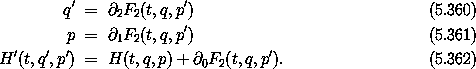
Recall the relations satisfied by an F2-type generating function:
If we require the new Hamiltonian to be zero, then F2 must satisfy the equation

So the solution of the problem is ``reduced'' to the problem of solving an n-dimensional partial differential equation for F2 with unspecified new (constant) momenta p'. This is the Hamilton-Jacobi equation, and in some cases we can solve it.
We can also attempt a somewhat less drastic method of solution. Rather than try to find an F2 that makes the new Hamiltonian identically zero, we can seek an F2-shaped function W that gives a new Hamiltonian that is solely a function of the new momenta. A system described by this form of Hamiltonian is also easy to solve. So if we set

and are able to solve for W, then the problem is essentially solved. In this case, the primed momenta are all constant and the primed positions are linear in time. This is an alternate form of the Hamilton-Jacobi equation.
These forms are related. Suppose that we have a W that satisfies the second form of the Hamilton-Jacobi equation (5.361). Then the F2 constructed from W

satisfies the first form of the Hamilton-Jacobi equation (5.360). Furthermore,

so the primed momenta are the same in the two formulations. But
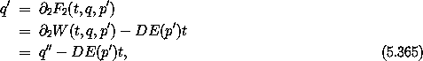
so we see that the primed coordinates differ by a term that is linear in time -- both p'(t) = p'0 and q'(t) = q'0 are constant. Thus we can use either W or F2 as the generating function, depending on the form of the new Hamiltonian we want.
Note that if H is time independent then we can often find a time-independent W that does the job. For time-independent W the Hamilton-Jacobi equation simplifies to

The corresponding F2 is then linear in time. Notice that an implicit requirement is that the energy can be written as a function of the new momenta alone. This excludes the possibility that the transformed phase-space coordinates q' and p' are simply initial conditions for q and p.
It turns out that there is flexibility in the choice of the function E. With an appropriate choice the phase-space coordinates obtained through the transformation generated by W are action-angle coordinates.
Exercise 5.23. Hamilton-Jacobi with F1
We have used an F2-type generating function to carry out the Hamilton-Jacobi transformations. Carry out the equivalent transformations with an F1-type generating function. Find the equations corresponding to equations (5.360), (5.361), and (5.365).
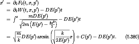
Consider the familiar time-independent Hamiltonian

We form the Hamilton-Jacobi equation for this problem:

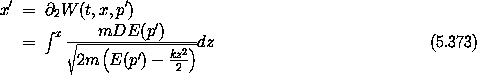
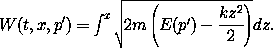
Using F2(t, x, p') = W(t, x, p') - E(p') t, we find

Writing this out explicitly yields

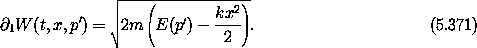
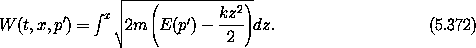
Integrating gives the desired W:
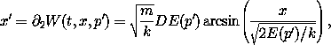
We can use either W or the corresponding F2 as the generating function. First, take W to be the generating function. We obtain the coordinate transformation by differentiating:
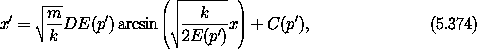
with some integration constant C(p'). Inverting this, we get the unprimed coordinate in terms of the primed coordinate and momentum:
The new Hamiltonian H' depends only on the momentum:

The equations of motion are just


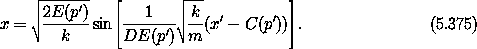
for initial conditions x'0 and p'0. If we plug these expressions for x'(t) and p'(t) into equation (5.374) we find
where the angular frequency is  = (k/m)1/2, the amplitude is
A = (2E(p')/k)1/2, and the phase is
= (k/m)1/2, the amplitude is
A = (2E(p')/k)1/2, and the phase is  = - t0 =
(x'0 - C(p'))/DE(p').
= - t0 =
(x'0 - C(p'))/DE(p').
We can also use F2 = W - E t as the generating function. The new Hamiltonian is zero, so both x' and p' are constant, but the relationship between the old and new variables is
Plugging in the solution x' = x'0 and p' = p'0 and solving for x, we find equation (5.378). So once again we see that the two approaches are equivalent.
It is interesting to note that the solution depends upon the constants E(p') and DE(p'), but otherwise the motion is not dependent in any essential way on what the function E actually is. The momentum p' is constant and the values of the constants are set by the initial conditions. Given a particular function E, the initial conditions determine p', but the solution can be obtained without further specifying the E function.
If we choose particular functions E we can get particular canonical transformations. For example, a convenient choice is simply

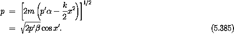
for some constant  that will be chosen later. We find

So we see that a convenient choice is = = (k/m)1/2,
so

with ß = (km)1/2. The new Hamiltonian is

The solution are just x' = t + x'0 and p' = p'0.
Substituting the expression for
x in terms of x' and p' into H(t, x, p) = H'(t, x', p'), we derive
The two transformation equations (5.382) and (5.383) are what we have called the polar-canonical transformation (equation 5.34). We have already shown that this transformation is canonical and that it solves the harmonic oscillator, but it was not derived. Here we have derived this transformation as a particular case of the solution of the Hamilton-Jacobi equation.
We can also explore other choices for the E function. For example, we could choose

Following the same steps as before, we find

So a convenient choice is again = , leaving
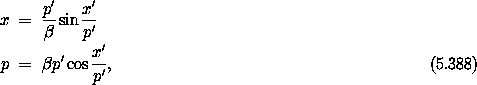
with ß = (km)1/4. By construction, this transformation is also canonical and also brings the harmonic oscillator problem into an easily solvable form:

The harmonic oscillator Hamiltonian has been transformed to what looks a lot like the Hamiltonian for a free particle. This is very interesting. Notice that whereas Hamiltonian (5.383) does not have a well defined Legendre transform to an equivalent Lagrangian, the ``free particle'' harmonic oscillator has a well defined Legendre transform:

Of course, there may be additional properties that make one choice more useful than others for particular applications.
Solve the Hamilton-Jacobi equation for the pendulum; investigate both the circulating and oscillating regions of phase space. (Note: This is a long story and requires some knowledge of elliptic functions.)
We can use the Hamilton-Jacobi equation to find canonical coordinates that solve the Kepler problem. This is an essential first step in doing perturbation theory for orbital problems.
In rectangular coordinates (x, y, z), the Kepler Hamiltonian is

where r2 = x2 + y2 + z2 and p2 = px2 + py2 + pz2. The Kepler problem describes the relative motion of two bodies; it is also encountered in the formulation of other problems involving orbital motion, such as the n-body problem.
We try a generating function of the form W(t; x, y, z; p'x, p'y, p'z). The Hamilton-Jacobi equation is then30
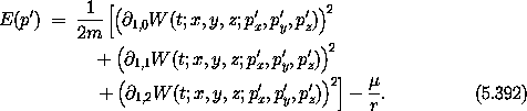
This is a partial differential equation in the three partial derivatives of W. We stare at it a while and give up.
Next we try converting to spherical coordinates. This is motivated by
the fact that the potential energy depends only on r. The Hamiltonian in
spherical coordinates (r,  , ), where is the
colatitude and is the longitude, is
, ), where is the
colatitude and is the longitude, is

The Hamilton-Jacobi equation is
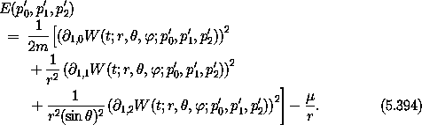
We can solve the Hamilton-Jacobi equation by successively isolating
the dependence on the various variables. Looking first at the
dependence, we see that, outside of W, appears only in one
partial derivative. If we write

then  1,2W(t; r, , ; p'0, p'1, p'2) = p'2, and then does not appear in
the remaining equation for f:
1,2W(t; r, , ; p'0, p'1, p'2) = p'2, and then does not appear in
the remaining equation for f:
Any function of the p'i could have been used as the coefficient of
in the generating function. This particular choice has the
nice feature that p'2 is the z component of the angular momentum.
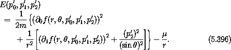
We can eliminate the dependence if we choose

and require that  be a solution to

We are free to choose the right-hand side to be any function of the
new momenta. This choice reflects the fact that the left-hand side is
non-negative. It turns out that p'1 is the total angular momentum.
This equation for can be solved by quadrature.
The remaining equation that determines R is

which also can be solved by quadrature.
Altogether the solution of the Hamilton-Jacobi equation reads
It is interesting that our solution to the Hamilton-Jacobi partial differential equation is of the form

Thus we have a separation-of-variables technique that involves writing the solution as a sum of functions of the individual variables. This might be contrasted with the separation-of-variables technique encountered in elementary quantum mechanics and classical electrodynamics, which uses products of functions of individual variables. However, integrable problems in classical mechanics are rare, so it would be incorrect to think of this method as a general solution method.
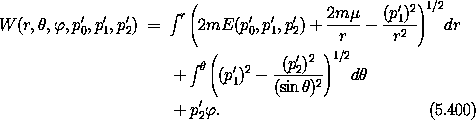
The coordinates q' = (q/ 0, q/ 1, q/ 2) conjugate to the momenta p' = [p'0, p'1, p'2] are
We are still free to choose the functional form of E. A convenient (and conventional) choice is

With this choice the momentum p'0 has dimensions of angular momentum, and the conjugate coordinate is an angle.
The Hamiltonian for the Kepler problem is reduced to

where n = m µ2 / (p'0)3 and where ß0, ß1, and ß2 are the initial values of the components of q'. Only one of the new variables changes with time.31
The solution to the Hamilton-Jacobi equation, the mixed-variable generating function that generates time evolution, is related to the action used in the variational principle. In particular, the time derivative of the generating function along realizable paths has the same value as the Lagrangian.
Let  2 (t) = F2(t, q(t), p'(t)) be the value of F2
along the paths q and p' at time t.
The derivative of 2 is
2 (t) = F2(t, q(t), p'(t)) be the value of F2
along the paths q and p' at time t.
The derivative of 2 is
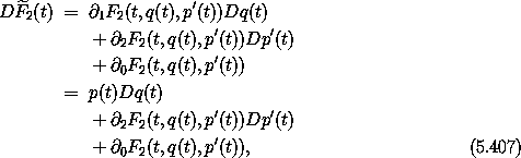
where we have used the relation for p in terms of F2 in the first term. Using the Hamilton-Jacobi equation (5.360), this becomes

On realizable paths we have Dp'(t) = 0, so along realizable paths the time derivative of F2 is the same as the Lagrangian along the path. The time integral of the Lagrangian along any path is the action along that path. This means that, up to an additive term that is constant on realizable paths but may be a function of the transformed phase-space coordinates q' and p', the F2 that solves the Hamilton-Jacobi equation has the same value as the Lagrangian action for realizable paths.
The same conclusion follows for the Hamilton-Jacobi equation formulated in terms of F1. Up to an additive term that is constant on realizable paths but may be a function of the transformed phase-space coordinates q' and p', the F1 that solves the corresponding Hamilton-Jacobi equation has the same value as the Lagrangian action for realizable paths.
Recall that a transformation given by an F2-type generating function is also given by an F1-type generating function related to it by a Legendre transform (see equation 5.195):

provided the transformations are nonsingular. In this case, both q' and p' are constant on realizable paths, so the additive constants that make F1 and F2 equal to the Lagrangian action differ by q' p'.
Exercise 5.25. Harmonic oscillator
Let's check this for the harmonic oscillator (of course).
a. Finish the integral (5.371):
Write the result in terms of the amplitude A = (2E(p')/k)1/2.
b. Check that this generating function gives the transformation
which is the same as equation (5.373) for a particular choice of the integration constant. The other part of the transformation is

with the same definition of A as before.
c. Compute the time derivative of the associated F2 along realizable paths (Dp'(t) = 0), and compare to the Lagrangian along realizable paths.
We define the function  (t1, q1, t2, q2) to be the value
of the action for a realizable path q such that q(t1) = q1 and
q(t2) = q2. So satisfies
(t1, q1, t2, q2) to be the value
of the action for a realizable path q such that q(t1) = q1 and
q(t2) = q2. So satisfies

For variations  that are not necessarily zero at the end times
and for realizable paths q, the variation of the action is
that are not necessarily zero at the end times
and for realizable paths q, the variation of the action is

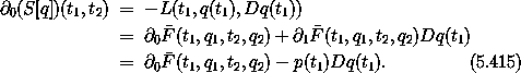
Alternatively, the variation of S[q] in equation (5.409) gives

Comparing equations (5.410) and
(5.411) and using the fact that the variation
is arbitrary, we find

The partial derivatives of with respect to the coordinate
arguments give the momenta. Abstracting off paths, we have

This looks a bit like the F1-type generating function relations, but here there are two times.
Given a realizable path q such that q(t1) = q1 and q(t2) = q2, we get the partial derivatives with respect to the time slots:


These are a pair of the Hamilton-Jacobi equations, computed at the
endpoints of the path.
Solving equations (5.413) for q2 and p2 as
functions of t2 and the initial state t1, q1, p1, we get
the time evolution of the system in terms of .
The function generates time evolution.
The function can be written in terms of the F2 or F1
that solves the Hamilton-Jacobi equation. We can compute time
evolution by using the F2 solution of the Hamilton-Jacobi equation
to express the state (t1, q1, p1) in terms of the constants q' and p' at a
given time t1. We can then perform a subsequent transformation back
from q' p' to the original state variables at a different time
t2, giving the state (t2, q2, p2). The composition of
canonical transformations is canonical. The generating function for
the composition is the difference of the generating functions for each
step:


which allows us to eliminate p'.
Exercise 5.26. Uniform acceleration
a. Compute the Lagrangian action, as a function of the
endpoints and times, for a uniformly accelerated particle. Use this
to construct the canonical transformation for time evolution from a
given initial state.
b. Solve the Hamilton-Jacobi equation for the uniformly accelerated particle, obtaining the F2 that makes the transformed Hamiltonian zero. Show that the Lagrangian action can be expressed as a difference of two applications of this F2.
30 Remember that 1,0 means the derivative with respect to the first coordinate position.
31 The canonical phase-space coordinates can be written in terms of the parameters that specify an orbit. We merely summarize the results; for further explanation see [36] or [38].
Assume we have a bound orbit with semimajor axis a,
eccentricity e, inclination i, longitude of ascending node
 , argument of pericenter , and mean anomaly M. The
three canonical momenta are
p'0 = (m µ a)1/2,
p'1 = (m µ a (1 - e2))1/2, and
p'2 = (m µ a (1 - e2))1/2 cos i.
The first momentum is related to the energy, the second momentum is
the total angular momentum, and the third momentum is the component of
the angular momentum in the
, argument of pericenter , and mean anomaly M. The
three canonical momenta are
p'0 = (m µ a)1/2,
p'1 = (m µ a (1 - e2))1/2, and
p'2 = (m µ a (1 - e2))1/2 cos i.
The first momentum is related to the energy, the second momentum is
the total angular momentum, and the third momentum is the component of
the angular momentum in the  direction. The conjugate
canonical coordinates are (q')0 = M, (q')1 = , and (q')2 = .
direction. The conjugate
canonical coordinates are (q')0 = M, (q')1 = , and (q')2 = .