 '(t) =
(t, q'(t), p'(t)) into (t) = (t, q(t), p(t)):
'(t) =
(t, q'(t), p'(t)) into (t) = (t, q(t), p(t)):
Although we have shown how to extend any point transformation of the configuration space to a canonical transformation, there are other ways to construct canonical transformations. How do we know if we have a canonical transformation? To test if a transformation is canonical we may use the fact that if the transformation is canonical, then Hamilton's equations of motion for the transformed system and the original system will be equivalent.
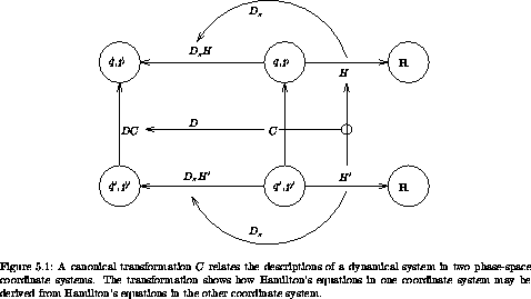
Consider a Hamiltonian H and a phase-space transformation C.
The transformation C transforms the phase-space path '(t) =
(t, q'(t), p'(t)) into (t) = (t, q(t), p(t)):

The rates of change of the phase-space coordinates are transformed by the derivative of the transformation

Let Ds be the phase-space derivative operator


for any realizable phase-space path .
The transformation is canonical if the equations of motion obtained from the new Hamiltonian are the same as those that could be obtained by transforming the equations of motion derived from the original Hamiltonian to the new coordinates:

Comparing equation (5.15) with this, we see


This condition must hold for any realizable phase-space path
'. Certainly this is true if the following condition holds
for every phase-space point:

Any transformation that satisfies equation (5.19) is a canonical transformation among phase-space representations of a dynamical system. In one phase-space representation the system's dynamics is characterized by the Hamiltonian H' and in the other by H. The idea behind this equation is illustrated in figure 5.1.
We can formalize this test as a program:
(define (canonical? C H Hprime)
(- (compose (phase-space-derivative H) C)
(* (D C) (phase-space-derivative Hprime))))
where phase-space-derivative, which was introduced in chapter 3, implements Ds. The transformation is canonical if these residuals are zero.
If a suitable Hamiltonian for the transformed system is obtained by composing H with the phase-space transformation, we obtain a more specific formula:

and a more specific test:
(define (compositional-canonical? C H)
(canonical? C H (compose H C)))
Using this test, we can verify that the polar-to-rectangular transformation satisfies the test for a canonical transformation on a general central field:
(print-expression
((compositional-canonical?
(F->CT p->r)
(H-central 'm (literal-function 'V)))
(up 't
(up 'r 'phi)
(down 'p_r 'p_phi))))
(up 0 (up 0 0) (down 0 0))
The residuals are zero so the transformation is canonical.
Exercise 5.2. Group properties
If we say that C is canonical with respect to Hamiltonians H and H' if and only if Ds H o C = DC · Ds H', then:
a. Show that the composition of canonical transformations is canonical. b. Show that composition of canonical transformations is associative. c. Show that the identity transformation is canonical. d. Show that there is an inverse for a canonical transformation and the inverse is canonical.
We have defined a canonical transformation as a transformation of phase-space coordinates for which Hamilton's equations transform appropriately. The conditions that a canonical transformation must satisfy (equations 5.19 or 5.20) involve the Hamiltonians. If the Hamiltonians transform by composition and the transformation is time independent, then we can tell if the phase-space transformation is canonical without further reference to the Hamiltonian.
First, we rewrite Hamilton's equations in a slightly different form. Hamilton's equations are constructed from the derivative of the Hamiltonian by rearranging the components and then negating some of them. We introduce a shuffle function that does this rearrangement:

The argument to  is a down tuple of components of the
derivative of a Hamiltonian-like function. The shuffle function is
linear. We also introduce a constant function:
is a down tuple of components of the
derivative of a Hamiltonian-like function. The shuffle function is
linear. We also introduce a constant function:

With these, Hamilton's equations can be expressed as

With and  the canonical
condition (5.20) can be rewritten
the canonical
condition (5.20) can be rewritten
The value of does not depend on its arguments, and for
time-independent transformations = DC ·
, so the canonical condition becomes

Applied to a particular phase-space state s this is

Let  be a function that takes a multiplier and produces a
linear transformation that multiplies the multiplier by the argument
to the linear transformation:
be a function that takes a multiplier and produces a
linear transformation that multiplies the multiplier by the argument
to the linear transformation:

Similarly, let * be a function that takes a multiplier and produces a
linear transformation that multiplies the argument to the linear
transformation by the multiplier:

Using and *, we can rewrite
condition (5.27) as

This condition is satisfied if

A time-independent transformation C is canonical, for Hamiltonians that transform by composition, if this condition on its derivative DC is satisfied.
Note that the condition (5.31) does not refer to the Hamiltonian. This is a remarkable result. Though we have assumed the Hamiltonians transform by composition with the transformation, we can decide whether a time-independent phase-space transformation preserves the dynamics of Hamilton's equation without further reference to the details of the dynamical system.
The test is implemented thus:
(define ((time-independent-canonical? C) s)
((- J-func
(compose (Phi ((D C) s))
J-func
(Phi* ((D C) s))))
(compatible-shape s)))
(define (J-func DH)
(up 0 (ref DH 2) (- (ref DH 1))))
(define ((Phi A) v) (* A v))
(define ((Phi* A) w) (* w A))
This procedure tests whether a composition of functions is the same
function as by computing their difference when applied
to a general typical argument.4
Here they are applied to a
structure with the shape of DH(s), for an arbitrary phase-space
state s.5
For example, consider the following polar-canonical transformation:

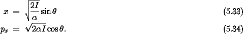
Here  is an arbitrary parameter. We define:
(define ((polar-canonical alpha) H-state)
(let ((t (time H-state))
(theta (coordinate H-state))
(I (momentum H-state)))
(let ((x (* (sqrt (/ (* 2 I) alpha)) (sin theta)))
(p_x (* (sqrt (* 2 alpha I)) (cos theta))))
(up t x p_x))))
And now we just run our test:
(print-expression
((time-independent-canonical? (polar-canonical 'alpha))
(up 't 'theta 'I)))
(up 0 0 0)
So the transformation is canonical.6
Of course, not every transformation we might try is
canonical. For example, we might try x = p sin  with px =
p cos . The implementation is7
with px =
p cos . The implementation is7
(define (a-non-canonical-transform H-state)
(let ((t (time H-state))
(theta (coordinate H-state))
(p (momentum H-state)))
(let ((x (* p (sin theta)))
(p_x (* p (cos theta))))
(up t x p_x))))
(print-expression
((time-independent-canonical? a-non-canonical-transform)
(up 't 'theta 'p)))
(up 0 (+ (* -1 p x8102) x8102) (+ (* p x8101) (* -1 x8101)))
So this transformation is not canonical.
The analysis of the harmonic oscillator illustrates the use of a general canonical transformation in the solution of a problem. The harmonic oscillator is a mathematical model of a simple spring-mass system. The Hamiltonian for a spring-mass system with mass m and spring constant k is

Hamilton's equations of motion are

giving the second-order system


and where A and  are determined by initial conditions.
Let's try our polar-canonical transformation C on the
harmonic oscillator. We substitute expressions (5.33) and
(5.34) for x and px in the Hamiltonian, getting our new
Hamiltonian:

If we choose = (km)1/2 then we obtain

and the new Hamiltonian no longer depends on the coordinate. Hamilton's equation for I is

so I is constant. The equation for is


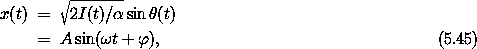
with the constant A = ( 2 I(t)/ )1/2.
So we have found the solution to the problem by making a canonical
transformation to new phase-space variables for which the solution is
easy and then transforming the solutions back to the original
variables.
Exercise 5.3. Trouble in Lagrangian world
Is there a Lagrangian L' that corresponds to the harmonic oscillator
Hamiltonian H'(t, , I) =  I? What could this possibly mean?
Exercise 5.4. Polar-canonical transformations
Let x, p and , I be two sets of canonically conjugate variables.
Consider transformations of the form x = ß I sin and
p = ß I cos . Determine all and ß for
which this transformation is compositional canonical.
Is the standard map a canonical transformation? Recall that the standard
map is: I' = I + K sin , with ' = + I', both
modulo 2 .
.
Condition (5.31) involves the composition of functions, all of which are linear transformations. Linear transformations can be represented in terms of matrices. A matrix representation is defined with respect to a basis. For incremental Hamiltonian states we organize the state components as a column matrix of time, the components of the coordinates, and the corresponding components of the momenta.
Let  and DC be matrix representations
of and (DC(s)), respectively, where s is
the arbitrary phase-space state at which the canonical condition is
being tested.
The matrix representation of *(DC(s)) is the transpose of DC. In terms of these matrix representations, the test for canonical
becomes
and DC be matrix representations
of and (DC(s)), respectively, where s is
the arbitrary phase-space state at which the canonical condition is
being tested.
The matrix representation of *(DC(s)) is the transpose of DC. In terms of these matrix representations, the test for canonical
becomes

We say that a transformation is symplectic if the matrix representation of its derivative satisfies this identity.
The matrix representation of the multiplier for the linear
transformation is . We can find
the multiplier for a linear transformation by taking the derivative of
the linear transformation and evaluating it at an arbitrary point:8
D( [ a, b, c ] ). We can obtain a matrix
representation with the utility s->m that takes a structure that represents a multiplier of
a linear transformation and returns a matrix representation of the
multiplier.9
The matrix depends only on the number of degrees of
freedom of the system. For example, the for a system with two
degrees of freedom is
(print-expression
(let* ((s (up 't (up 'x 'y) (down 'px 'py)))
(s* (compatible-shape s)))
(s->m s* ((D J-func) s*) s*)))
(matrix-by-rows (list 0 0 0 0 0)
(list 0 0 0 1 0)
(list 0 0 0 0 1)
(list 0 -1 0 0 0)
(list 0 0 -1 0 0))
In terms of matrix representations, the test that a transformation is symplectic is
(define ((symplectic? C) s)
(let ((s* (compatible-shape s)))
(let ((J (s->m s* ((D J-func) s*) s*))
(DCs (s->m s* ((D C) s) s)))
(- J (* DCs J (m:transpose DCs))))))
For example, we can verify that the point transformation derived from the coordinate transformation p->r is symplectic:
(print-expression
((symplectic? (F->CT p->r))
(up 't
(up 'r 'varphi)
(down 'p_r 'p_varphi))))
(matrix-by-rows (list 0 0 0 0 0)
(list 0 0 0 0 0)
(list 0 0 0 0 0)
(list 0 0 0 0 0)
(list 0 0 0 0 0))
There is a further simplification available. The elements of the
first row and the first column of the matrix representation of
are all zeros. Thus we need to consider only the
submatrix associated with the coordinates and the momenta.
The qp submatrix10
of dimension 2n× 2n of the matrix is called
the symplectic unit for n degrees of freedom:

The matrix Jn satisfies the following identities:

A 2n× 2n matrix A that satisfies the relation

is called a symplectic matrix.
Here is an alternate test for whether a transformation is symplectic:
(define ((symplectic-transform? C) s)
(symplectic-matrix?
(qp-submatrix
(s->m (compatible-shape s)
((D C) s)
s))))
(define (symplectic-matrix? M)
(let ((2n (m:dimension M)))
(let ((J (symplectic-unit (quotient 2n 2))))
(- J (* M J (m:transpose M))))))
The procedure symplectic-transform? returns a zero matrix if and only if the transformation being tested passes the symplectic matrix test. An appropriate symplectic unit matrix of a given size is produced by the procedure symplectic-unit.
The point transformations are symplectic. For example,
(print-expression
((symplectic-transform? (F->CT p->r))
(up 't
(up 'r 'theta)
(down 'p_r 'p_theta))))
(matrix-by-rows (list 0 0 0 0)
(list 0 0 0 0)
(list 0 0 0 0)
(list 0 0 0 0))
Exercise 5.6. Symplectic matrices
Let A be a symplectic matrix: Jn = A Jn
AT . Show that AT and A-1 are
symplectic.
Exercise 5.7. Whittaker transform
Shew that the transformation
q = log ( (1/q') sin p' ) with
p = q' cot p' is symplectic.
We have found that a time-independent transformation (involving the coordinates and conjugate momenta, but not the time) is canonical if the derivative of the transformation is symplectic. Let's return to the calculation of the symplectic condition, but now allow explicit time dependence in the transformation equations.
If the transformation is time dependent, then it turns out that H o C does not make a suitable H'. Instead, we assume

and look for conditions on K and C that guarantee the transformation is canonical. Equation (5.25), the condition that a transformation is canonical, becomes

This condition is satisfied if the following two conditions are satisfied:


Condition (5.52) is the condition that C is a
symplectic transformation. Condition (5.53) is an
auxiliary condition on K. This condition does not actually depend
on the Hamiltonian H because the constant value of
does not depend on the argument. The time component is always
satisfied; only the coordinate and momentum components of this
condition constrain K. Evaluated at a particular state s (with
compatible shape s*), the condition on K is

explicitly showing that the Hamiltonian H does not enter.
Thus we can conclude that a time-dependent transformation is canonical if its position-momentum part is symplectic and if we form the new Hamiltonian by adding an appropriate piece. Note that we have not proven that the position-momentum part must be symplectic. Rather, we have shown that if this part is symplectic then the Hamiltonian must be modified in an appropriate way.
As a program, the test for K is
(define ((canonical-K? C K) s)
(let ((s* (compatible-shape s)))
(- (T-func s*)
(+ (* ((D C) s) (J-func ((D K) s)))
(((partial 0) C) s)))))
Consider a time-dependent transformation to uniformly rotating coordinates:


As a program this is
(define ((rotating n) state)
(let ((t (time state))
(q (coordinate state)))
(let ((x (ref q 0))
(y (ref q 1))
(z (ref q 2)))
(up (+ (* (cos (* n t)) x) (* (sin (* n t)) y))
(- (* (cos (* n t)) y) (* (sin (* n t)) x))
z))))
The extension of this transformation to a phase-space transformation is
(define (C-rotating Omega) (F->CT (rotating Omega)))
We first verify that the position-momentum part of this time-dependent transformation is symplectic:
(print-expression
((symplectic-transform? (C-rotating 'Omega))
(up 't
(up 'x 'y 'z)
(down 'px 'py 'pz))))
(matrix-by-rows (list 0 0 0 0 0 0)
(list 0 0 0 0 0 0)
(list 0 0 0 0 0 0)
(list 0 0 0 0 0 0)
(list 0 0 0 0 0 0)
(list 0 0 0 0 0 0))
For this transformation the appropriate correction to the Hamiltonian is

which is the rate of rotation of the coordinate system multiplied by the angular momentum. The justification for this will be given in section 5.6. The implementation is
(define ((K Omega) s)
(let ((q (coordinate s)) (p (momentum s)))
(let ((x (ref q 0)) (y (ref q 1))
(px (ref p 0)) (py (ref p 1)))
(* -1 Omega (- (* x py) (* y px))))))
Applying the test, we find:
(print-expression
((canonical-K? (C-rotating 'Omega) (K 'Omega))
(up 't
(up 'x 'y 'z)
(down 'p_x 'p_y 'p_z))))
(up 0 (up 0 0 0) (down 0 0 0))
The residuals are zero so this K completes the canonical transformation.
A transformation is symplectic if the qp part of the transformation has a symplectic derivative. This condition can be written simply in terms of Poisson brackets.
The Poisson bracket can be written in terms of :

as can be seen by writing out the components.
We break the transformation C into position and momentum parts:

In terms of the individual component functions, the symplectic condition (5.46) is
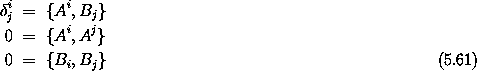
where  ij is one if i = j and zero otherwise.
These are called the fundamental Poisson brackets. If
a transformation satisfies these
Poisson bracket relations then it is symplectic.
ij is one if i = j and zero otherwise.
These are called the fundamental Poisson brackets. If
a transformation satisfies these
Poisson bracket relations then it is symplectic.
We have found that a time-dependent transformation is canonical if its position-momentum part is symplectic and we modify the Hamiltonian by the addition of a suitable K. We can rewrite these conditions in terms of Poisson brackets. If the Hamiltonian is

the transformation will be canonical if the coordinate-momentum transformation satisfies the fundamental Poisson brackets, and K satisfies:

Fill in the details to show that the symplectic condition (5.31) is equivalent to the fundamental Poisson brackets (5.61) and that the condition on K (5.53) is equivalent to the Poisson bracket condition on K (5.63).
4 It is in principle impossible to determine in general if two
functions are the same, but in this case, since (DC(s)) is
linear, this test is valid.
5 The shape of DH(s) is a compatible shape to the shape of s: if they are multiplied the result is a real number. The procedure compatible-shape takes any structure and produces another structure that is guaranteed to multiply with the given structure to produce a real number. The structure produced is filled with unique real literals, so if the residual is zero then the functions are the same.
6 Actually, for I = 0 the transform is not well defined and so it is not compositional canonical for that value. This transformation is ``locally compositional canonical'' in that it is compositional canonical for nonzero values of I. We will ignore this essentially topological problem.
7 The mysterious symbols such as x8102 are unique real literals introduced to test functional equalities. That they appear in a residual demonstrates that the equality is invalid.
8 The derivative of a linear transformation is a constant function, independent of the argument.
9 The procedure s->m takes three arguments: (s->m s* A s). The s* and s specify the shapes of objects that multiply A on the left and right to give a numerical value; these specify the basis.
10 The qp submatrix of a 2n + 1-dimensional square matrix is the 2n-dimensional matrix obtained by deleting the first row and the first column of the given matrix. This can be computed by:
(define (qp-submatrix m)
(m:submatrix m 1 (m:num-rows m) 1 (m:num-cols m)))