 , J) = f(J). We add some small
additional effect described by the term H1 in the Hamiltonian
, J) = f(J). We add some small
additional effect described by the term H1 in the Hamiltonian
How does this picture change if we add additional effects?
One peculiar feature of the orbits in integrable systems is that there are continuous families of periodic orbits. The initial angles do not matter; the frequencies depend only on the actions. Contrast this with our earlier experience with surfaces of section in which periodic points are isolated, and associated with island chains. Poincaré and Birkhoff investigated periodic orbits of near-integrable systems, and found that typically for each rational rotation number there are a finite number of periodic points, half of which are linearly stable and half linearly unstable. Here we show how to construct the Poincaré-Birkhoff periodic points.
Consider an integrable system described in action-angle coordinates by
the Hamiltonian H0(t, , J) = f(J). We add some small
additional effect described by the term H1 in the Hamiltonian

An example of such a system is the periodically driven pendulum with small-amplitude drive. For zero-amplitude drive the driven pendulum is integrable, but not for small drive. Unfortunately, we do not yet have the tools to develop action-angle coordinates for the pendulum. A simpler problem that is already in action-angle form is the driven rotor, which is just the driven pendulum with gravity turned off. We can implement this by turning our driven pendulum on its side, making the plane of the pendulum horizontal. A Hamiltonian for the driven rotor is

where A is the amplitude of the drive with frequency  , m
is the mass of the bob, and l is the length of the rotor. For zero
amplitude, the Hamiltonian is already in action-angle form in that it
depends only on the momentum p and the coordinate is an
angle.
, m
is the mass of the bob, and l is the length of the rotor. For zero
amplitude, the Hamiltonian is already in action-angle form in that it
depends only on the momentum p and the coordinate is an
angle.
For an integrable system, the map generated on the surface of section is of the form (4.39). With the addition of a small perturbation to the Hamiltonian, small corrections are added to the map
Both the map T and the perturbed map T are area
preserving because the maps are generated as surfaces of section for
Hamiltonian systems.
are area
preserving because the maps are generated as surfaces of section for
Hamiltonian systems.
Suppose we are interested in determining whether periodic orbits of a
particular rational rotation number  (
( (0)) = j/k exist in
some interval of the action
(0)) = j/k exist in
some interval of the action  < (0) < ß. If the
rotation number is strictly monotonic in this interval and orbits with
the rotation number ((0)) occur in this interval for the
unperturbed map T, then by a simple construction we can show that
periodic orbits with this rotation number also exist for T
for sufficiently small .
< (0) < ß. If the
rotation number is strictly monotonic in this interval and orbits with
the rotation number ((0)) occur in this interval for the
unperturbed map T, then by a simple construction we can show that
periodic orbits with this rotation number also exist for T
for sufficiently small .
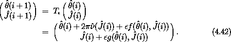
If a point is periodic for rational rotation number ((0)) =
j/k, with relatively prime j and k, we expect k distinct images
of the point to appear on the section. So if we consider the kth
iterate of the map then the point is a fixed point of the map. For
rational rotation number j/k the map Tk has a fixed point for
every initial angle.
The rotation number of the map T is strictly monotonic. Suppose for
definiteness we assume the rotation number ((0)) increases with
(0). For some * such that < * <
ß the
rotation number is j/k, and ( *, *) is a fixed
point of
Tk for any initial
*. For * the rotation number of Tk is zero. The
rotation number of the map T is monotonically increasing so for (0)
> * the rotation number of Tk is positive, and for (0) <
* the rotation number of Tk is negative, as long as (0) is
not too far from *. See figure 4.12.
*, *) is a fixed
point of
Tk for any initial
*. For * the rotation number of Tk is zero. The
rotation number of the map T is monotonically increasing so for (0)
> * the rotation number of Tk is positive, and for (0) <
* the rotation number of Tk is negative, as long as (0) is
not too far from *. See figure 4.12.
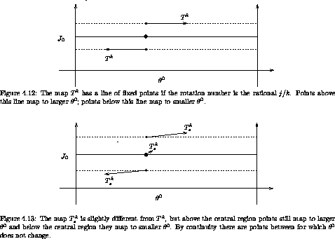
Now consider the map Tk. In general, for small
, points map to slightly different points under T
than they do under T, but not too different. So we can expect that
there is still some interval near * such that for (0) in the
upper end of the interval, Tk maps points to larger
0, and for points in the lower end of the interval,
Tk maps points
to smaller 0. If this is the case then
for every (0) there is a point somewhere in the interval, some
+((0)), for which 0 does not change, by
continuity. These are not fixed points because the momentum J0
generally changes. See figure 4.12.
The map is continuous, so we can expect that + is a continuous
function of the 0. As we let 0 vary through 2 ,
this function is either periodic or not. That it must be periodic is
a consequence of area preservation.13
So the set of points that do not change 0 under Tk
form some periodic function of 0. Call this curve C0.
See figure 4.14.
,
this function is either periodic or not. That it must be periodic is
a consequence of area preservation.13
So the set of points that do not change 0 under Tk
form some periodic function of 0. Call this curve C0.
See figure 4.14.
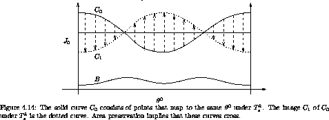
The map Tk takes the curve C0 to another curve C1
that, like C0, is continuous and periodic. The two curves C0
and C1 must cross each other, as a consequence of area
preservation. How do we see this? Typically, there is a lower
boundary or upper boundary in J0 for the evolution. In some
situations, we have such a lower boundary because J0 cannot be
negative. For example, in action-angle variables for motion near an
elliptic fixed point we will see that the action is the area enclosed
on the phase plane, which cannot be negative. For others, we might
use the fact that there are invariant curves for large positive or
negative J0. In any case, suppose there is such a barrier B.
Then, the area of the region between the barrier and C0 must be
equal to the area of the image of this region, which is the region
between the barrier and C1. So if at any point the two
curves C0 and C1 do not coincide, then they must cross to
contain the same area. In fact, they must cross an even number of
times: they are both periodic, so if they cross once they must
cross again to get back to the same side they started on. The points
at which the curves C0 and C1 cross are fixed points because the
angle does not change (that is what it means to be on C0) and the
action does not change (that is what it means for C0 and C1 to
be the same at this point). So we have deduced that there must be an
even number of fixed points of Tk. For each fixed point
of Tk there are k images of this fixed point generated on the
surface of section for the map T.
Each of these image points is a periodic point of the map T.
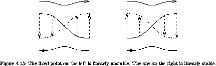
We can deduce the stability of these fixed points of Tk
just from the
construction. The fixed points come in two types, elliptic and
hyperbolic. An elliptic fixed point appears where the flow is around
the fixed point: the map from C0 to C1 can be continued along
the background flow to make a closed curve. A hyperbolic fixed point
appears where in following the map from C0 to C1 we enter the
background flow in such a way as to leave the fixed point. So just
from the way the arrows connect we can determine the character of the
fixed point. See figure 4.15.
As we develop a Poincaré section, we find that some orbits leave traces that circulate around the stable fixed points, resulting in the Poincaré-Birkhoff islands. If we look at a particular island we see that orbits in the island circulate around the fixed point at a rate that is monotonically dependent upon the distance from the fixed point. In the vicinity of the fixed point the evolution is governed by a twist map. So the entire Poincaré-Birkhoff construction can be carried out again. We expect that there will be concentric families of stable periodic points surrounded by islands and separated by separatrices emanating from unstable periodic points. Around each of these stable periodic orbits, the construction is repeated. So the Poincaré-Birkhoff construction is recursive, leading to the development of an infinite hierarchy of structure.
There are so many conditions in our construction of the fixed points
that one might be suspicious. We can make the construction more
convincing by actually computing the various pieces for a specific
problem. Consider the periodically driven rotor, with
Hamiltonian (4.41). We set m = 1 kg,
l = 1 m,
A = 0.1 m, = 4.2 (9.8)1/2 rad s-1.
We call points that map to the same angle ``radially mapping points.'' We find them with a simple bisection:
(define (radially-mapping-points Tmap Jmin Jmax phi eps)
(bisect
(lambda (J)
((principal-value pi)
(- phi (Tmap phi J (lambda (phip Jp) phip) list))))
Jmin Jmax eps))
The procedure Tmap implements some map, which may be an iterate of some more primitive map. We give the procedure an angle phi to study, a range of actions Jmin to Jmax to search, and a tolerance eps for the solution.
We make a plot of the curves C0 (of initial conditions that map radially) and C1 (the image of C0) with an appropriate piece of wrapper code.
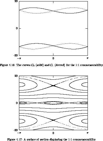
In figure 4.16 we show the Poincaré-Birkhoff construction of the fixed points for the driven rotor. These particular curves are constructed for the two 1:1 commensurabilities between the rotation and the drive. One set of fixed points is constructed for each sense of rotation. The corresponding section is in figure 4.17. We see that the section shows the existence of fixed points exactly where the Poincaré-Birkhoff construction shows the crossing of the curves C0 and C1. Indeed, the nature of the fixed point is clearly reflected in the relative configuration of the C0 and C1 curves.
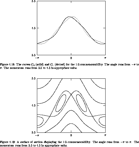
In figure 4.18 we show the result for a rotation number of 1/3. The curves are the radially mapping points for the third iterate of the section map (solid) and the images of these points (dotted). These curves are distorted by their proximity to the 1:1 islands shown in figure 4.17. The corresponding section is shown in figure 4.19.
Exercise 4.7. Computing the Poincaré-Birkhoff construction
Consider figure 3.27. Find the fixed points
for the three major island chains, using the Poincaré-Birkhoff
construction.
13 If + were not periodic in 0 then it would
have to spiral. Suppose it spirals. The region enclosed by two
successive turns of the spiral is mapped to a region between successive
turns of the spiral further down the spiral. The map preserves area,
so the spiral cannot get tighter and tighter, but must progress infinitely down the
cylinder. This is impossible because of the twist condition:
sufficiently far down the cylinder the rotation number is too different
to allow the angle to be the same under Tk. So
+ does not spiral.