
The momenta are given by momentum state functions of the time, the coordinates, and the velocities.1 Locally, we can find inverse functions that give the velocities in terms of the time, the coordinates, and the momenta. We can use this inverse function to represent the state in terms of the coordinates and momenta rather than the coordinates and velocities. The equations of motion when recast in terms of coordinates and momenta are called Hamilton's canonical equations.
We present three derivations of Hamilton's equations. The first derivation is guided by the strategy outlined above and uses nothing more complicated than implicit functions and the chain rule. The second derivation first abstracts a key part of the first derivation and then applies the more abstract machinery to derive Hamilton's equations. The third uses the action principle.
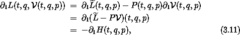
Lagrange's equations give us the time derivative of the momentum p on a path q:

To eliminate Dq we need to solve equation (3.2) for Dq in terms of p.
Let  be the function that gives the velocities in terms of
the time, coordinates, and momenta. Defining is a problem
of functional inverses. To prevent confusion we use names for the
variables that have no mnemonic significance. Let
be the function that gives the velocities in terms of
the time, coordinates, and momenta. Defining is a problem
of functional inverses. To prevent confusion we use names for the
variables that have no mnemonic significance. Let


So and  2 L are inverses on the third argument position:

The Lagrange equation (3.1) can be rewritten in
terms of p using :

We can also use to rewrite
equation (3.2) as an equation for Dq in terms
of t, q and p:

Equations (3.7) and (3.8) give the rate of change of q and p along realizable paths as functions of t, q, and p along the paths.
Though these equations fulfill our goal of expressing the equations of motion entirely in terms of coordinates and momenta, we can find a more convenient representation. Define the function

which is the Lagrangian reexpressed as a function of time,
coordinates, and momenta.2
For the equations of motion we need
1 L evaluated with the appropriate arguments. Consider

where we used the chain rule in the first step and the inverse
property (3.5) of in the second step. Introducing the momentum selector3
P(t, q, p) = p, and using the property 1 P = 0, we have
where the Hamiltonian H is defined by4

Using the algebraic result (3.11), the Lagrange equation (3.7) for Dp becomes

The equation for Dq can also be written in terms of H. Consider

To carry out the derivative of  we write it out
in terms of L:
we write it out
in terms of L:

again using the inverse property (3.5) of . So, putting equations
(3.14) and (3.15) together,
we obtain

Using the algebraic result (3.16), equation (3.8) for Dq becomes

Equations (3.13) and (3.17) give the derivatives of the coordinate and momentum path functions at each time in terms of the time, and the coordinates, and momenta at that time. These equations are known as Hamilton's equations:5

The first equation is just a restatement of the relationship of the momenta to the velocities in terms of the Hamiltonian and holds for any path, whether or not it is a realizable path. The second equation holds only for realizable paths.
Hamilton's equations have an especially simple and symmetrical form. Just as Lagrange's equations are constructed from a real-valued function, the Lagrangian, Hamilton's equations are constructed from a real-valued function, the Hamiltonian. The Hamiltonian function is6

The Hamiltonian has the same value as the energy function  (see equation 1.140), except that the
velocities are expressed in terms of time, coordinates, and momenta by
:
(see equation 1.140), except that the
velocities are expressed in terms of time, coordinates, and momenta by
:

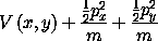
Let's try something simple: the motion of a particle of mass m with potential energy V(x, y). A Lagrangian is

To form the Hamiltonian we find the momenta p = 2 L(t,
q, v):
px = m vx and py = m vy. Solving for the velocities
in terms of the momenta is easy here: vx = px/m and vy =
py/m. The Hamiltonian is H(t, q, p) = pv - L(t, q, v), with v reexpressed in
terms of (t, q, p):

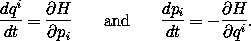
The kinetic energy is a homogeneous quadratic form in the velocities, so the energy is T + V and the Hamiltonian is the energy expressed in terms of momenta rather than velocities. Hamilton's equations for Dq are

Note that these equations merely restate the relation between the momenta and the velocities. Hamilton's equations for Dp are

The rate of change of the linear momentum is minus the gradient of the potential energy.
Exercise 3.1. Deriving Hamilton's equations
For each of the following Lagrangians derive the Hamiltonian and
Hamilton's equations. These problems are simple enough to do by hand.
a. A Lagrangian for a planar pendulum:
L(t,  ,
,  ) = (1/2) m l2 2 + m g l cos .
b. A Lagrangian for a particle of mass m with a
two-dimensional
potential energy: V(x, y) = (x2 + y2)/2 + x2 y - y3/3 is L(t; x, y;
 ,
,  ) = (1/2) m (2 + 2) - V(x, y).
c. A Lagrangian for a particle of mass m constrained to move
on a sphere of radius R: L(t; ,  ; ,
; ,
 ) = (1/2) m R2 (2 + ( sin
)2), where is the colatitude and is the
longitude on the sphere.
) = (1/2) m R2 (2 + ( sin
)2), where is the colatitude and is the
longitude on the sphere.
Exercise 3.2. Sliding pendulum
For the pendulum with a sliding support (see
exercise 1.20), derive a Hamiltonian
and Hamilton's equations.
Given a coordinate path q and a Lagrangian L, the corresponding
momentum path p is given by equation (3.2).
Equation (3.17) expresses the same relationship in
terms of the corresponding Hamiltonian H. That these relations are
valid for any path, whether or not it is a realizable path, allows us
to abstract to arbitrary velocity and momentum at a moment. At a
moment, the momentum p for the state tuple ( t, q, v ) is p =
2 L(t, q, v). We also have v = 2 H(t, q, p). In
the Lagrangian formulation the state of the system at a moment can be
specified by the local state tuple ( t, q, v ) of time, generalized
coordinates, and generalized velocities. Lagrange's equations
determine a unique path emanating from this state. In the Hamiltonian
formulation the state can be specified by the tuple ( t, q, p ) of
time, generalized coordinates, and generalized momenta. Hamilton's
equations determine a unique path emanating from this state. The
Lagrangian state tuple ( t, q, v ) encodes exactly the same
information as the Hamiltonian state tuple ( t, q, p ); we need a
Lagrangian or a Hamiltonian to relate them. The two formulations are
equivalent in that the same coordinate
path emanates from them for equivalent initial states.
The Lagrangian state derivative is constructed from the Lagrange equations by solving for the highest-order derivative and abstracting to arbitrary positions and velocities at a moment.7 The Lagrangian state path is generated by integration of the Lagrangian state derivative given an initial Lagrangian state ( t, q, v ). Similarly, the Hamiltonian state derivative can be constructed from Hamilton's equations by abstracting to arbitrary positions and momenta at a moment. Hamilton's equations are a set of first-order differential equations in explicit form. The Hamiltonian state derivative can be directly written in terms of them. The Hamiltonian state path is generated by integration of the Hamiltonian state derivative given an initial Hamiltonian state ( t, q, p ). If these state paths are obtained by integrating the state derivatives with equivalent initial states, then the coordinate path components of these state paths are the same and satisfy the Lagrange equations. The coordinate path and the momentum path components of the Hamiltonian state path satisfy Hamilton's equations. The Hamiltonian formulation and the Lagrangian formulation are equivalent.
Given a path q, the Lagrangian state path and the Hamiltonian state paths
can be deduced from it. The Lagrangian state path  [q] can be
constructed from a path q simply by taking derivatives. The
Lagrangian state path satisfies:
[q] can be
constructed from a path q simply by taking derivatives. The
Lagrangian state path satisfies:

The Lagrangian state path is uniquely determined by the path q.
The Hamiltonian state path  L[q] can also be constructed from the
path q but the construction requires a Lagrangian. The
Hamiltonian state path satisfies
L[q] can also be constructed from the
path q but the construction requires a Lagrangian. The
Hamiltonian state path satisfies

The Hamiltonian state tuple is not uniquely determined by the path q because it depends upon our choice of Lagrangian, which is not unique.
The 2n-dimensional space whose elements are labeled by the n generalized coordinates qi and the n generalized momenta pi is called the phase space. The components of the generalized coordinates and momenta are collectively called the phase-space components.8 The dynamical state of the system is completely specified by the phase-space state tuple ( t, q, p ), given a Lagrangian or Hamiltonian to provide the map between velocities and momenta.
Hamilton's equations are a system of first-order ordinary differential equations. A procedural formulation of Lagrange's equations as a first-order system was presented in section 1.7. The following formulation of Hamilton's equations is analogous:
(define ((Hamilton-equations Hamiltonian) q p)
(let ((H-state-path (qp->H-state-path q p)))
(- (D H-state-path)
(compose (phase-space-derivative Hamiltonian)
H-state-path))))
The Hamiltonian state derivative is computed as follows:
(define ((phase-space-derivative Hamiltonian) H-state)
(up 1
(((partial 2)Hamiltonian) H-state)
(- (((partial 1)Hamiltonian) H-state))))
The state in the Hamiltonian formulation is composed of the time, the coordinates, and the momenta. We call this an H-state, to distinguish it from the state in the Lagrangian formulation. We can select the components of the Hamiltonian state with the selectors time, coordinate, momentum. We construct Hamiltonian states from their components with up. The first component of the state is time, so the first component of the state derivative is one, the time rate of change of time. Given procedures q and p implementing coordinate and momentum path functions, the Hamiltonian state path can be constructed with the following procedure:
(define ((qp->H-state-path q p) t)
(up t (q t) (p t)))
The Hamilton-equations procedure returns the residuals of Hamilton's equations for the given paths.
For example, a procedure implementing the Hamiltonian for a point mass with potential energy V(x, y) is
(define ((H-rectangular m V) H-state)
(let ((q (coordinate H-state))
(p (momentum H-state)))
(+ (/ (square p) (* 2 m))
(V (ref q 0) (ref q 1)))))
Hamilton's equations are9
(show-expression
(((Hamilton-equations
(H-rectangular
'm
(literal-function 'V (-> (X Real Real) Real))))
(up (literal-function 'x) (literal-function 'y))
(down (literal-function 'p_x) (literal-function 'p_y)))
't))
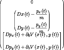
The zero in the first element of the structure of Hamilton's equation residuals is just the tautology that time advances uniformly: the time function is just the identity, so its derivative is one and the residual is zero. The equations in the second element of the structure relate the coordinate paths and the momentum paths. The equations in the third element give the rate of change of the momenta in terms of the applied forces.
Exercise 3.3. Computing Hamilton's equations
Check your answers to exercise 3.1 with the
Hamilton-equations procedure.
The Legendre transformation abstracts a key part of the process of transforming from the Lagrangian to the Hamiltonian formulation of mechanics -- the replacement of functional dependence on generalized velocities with functional dependence on generalized momenta. The momentum state function is defined as a partial derivative of the Lagrangian, a real-valued function of time, coordinates, and velocities. The Legendre transformation provides an inverse that gives the velocities in terms of the momenta: we are able to write the velocities as a partial derivative of a different real-valued function of time, coordinates, and momenta.10
Given a real-valued function F, if we can find a real-valued function G such that DF = (DG)-1, then we say that F and G are related by a Legendre transform.
Locally, we can define the inverse function11
of DF so that DF o = I, where I is the identity
function I(w) = w. Consider the composite function  =
F o . The derivative of is
=
F o . The derivative of is

Using the product rule and DI = 1, we have


The integral is determined up to a constant of integration. If we define


The function G has the desired property that DG is the inverse
function of DF. The derivation just given applies
equally well if the arguments of F and G have multiple components.
Given a relation w = DF(v) for some given function F, then
v = DG(w) for G = I - F o , where is the inverse
function of DF provided it exists.
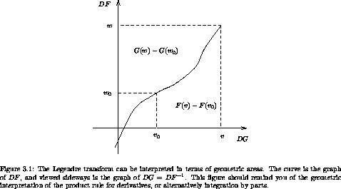
A picture may help (see figure 3.1). The curve is the graph of the function DF. Turned sideways, it is also the graph of the function DG, because DG is the inverse function of DF. The integral of DF from v0 to v is F(v) - F(v0); this is the area below the curve from v0 to v. Likewise, the integral of DG from w0 to w is G(w) - G(w0); this is the area to the left of the curve from w0 to w. The union of these two regions has area w v - w0 v0. So


The left-hand side depends only on the point labeled by w and v and the right-hand side depends only on the point labeled by w0 and v0, so these must be constant, independent of the variable endpoints. So as the point is changed the combination G(w) + F(v) - wv is invariant. Thus

with constant C. The requirement for G depends only on DG so we can choose to define G with C = 0.
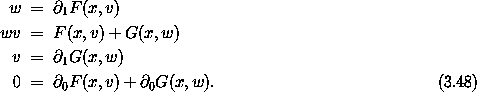
Let F be a real-valued function of two arguments and

If we can find a real-valued function G such that

we say that F and G are related by a Legendre transformation, that the second argument in each function is active, and that the first argument is passive in the transformation.
If the function 1 F can be locally inverted with
respect to the second argument we can define


where W = I1 is the selector function for the second argument.
For the active arguments the derivation goes through as before. The first argument to F and G is just along for the ride -- it is a passive argument. Let


We can check that G has the property = 1
G by carrying out the derivative:


as required. The active argument may have many components.
The partial derivatives with respect to the passive
arguments are related in a remarkably simple way. Let's calculate the
derivative 0 G in pieces. First,

because 0 W = 0. To calculate
0 we must supply arguments:

Putting these together, we find

The calculation is unchanged if the passive argument has many components.
We can write the Legendre transformation more symmetrically:
The last relation is not as trivial as it looks, because x enters the equations connecting w and v. With this symmetrical form, we see that the Legendre transform is its own inverse.
Exercise 3.4. Simple Legendre transforms
For each of the following functions, find the function that is related
to the given function by the Legendre transform on the indicated
active argument.
Show that the Legendre transform relations hold for your solution,
including the relations among passive arguments, if any.
a. F(x) = a x + b x2, with no passive arguments.
b. F(x, y) = a sin x cos y, with x active.
c. F(x, y, , ) = x 2 + 3 + y 2, with and active.
We can use the Legendre transformation with the Lagrangian playing the role of F and with the generalized velocity slot playing the role of the active argument. The Hamiltonian plays the role of G with the momentum slot active. The coordinate and time slots are passive arguments.
The Lagrangian L and the Hamiltonian H are related by a Legendre transformation:


Presuming it exists, we can define the inverse of 2 L
with respect to the last argument:


These relations are purely algebraic in nature.
On a path q we have the momentum p:

and from the definition of we find


This relation is purely algebraic and is valid for any path. The passive equation (3.53) gives

but the left-hand side can be rewritten using the Lagrange equations, so

This equation is valid only for realizable paths, because we used the Lagrange equations to derive it. Equations (3.58) and (3.60) are Hamilton's equations.
The remaining passive equation is

This passive equation says that the Lagrangian has no explicit time
dependence (0 L = 0) if and only if the
Hamiltonian has no explicit time dependence (0 H =
0). We have found that if the Lagrangian has no explicit time
dependence, then energy is conserved. So if the Hamiltonian has no
explicit time dependence then it is a conserved quantity.
Exercise 3.5.
Using Hamilton's equations, show directly that the Hamiltonian is a
conserved quantity if it has no explicit time dependence.
We cannot implement the Legendre transform in general because it involves finding the functional inverse of an arbitrary function. However, many physical systems can be described by Lagrangians that are quadratic forms in the generalized velocities. For such functions the generalized momenta are linear functions of the generalized velocities, and thus explicitly invertible.
More generally, we can compute a Legendre transformation for polynomial functions where the leading term is a quadratic form:

We can assume M is symmetric,12 because it defines a quadratic form. We can find linear expressions for w as

So if M is invertible we can solve for v in terms of w.
Thus we may define a function such that

and we can use this to compute the value of the function G:

We implement the Legendre transform for quadratic functions by the procedure13
(define (Legendre-transform F)
(let ((w-of-v (D F)))
(define (G w)
(let ((z (dual-zero w)))
(let ((M ((D w-of-v) z))
(b (w-of-v z)))
(let ((v (/ (- w b) M)))
(- (* w v) (F v))))))
G))
The procedure Legendre-transform takes a procedure of one
argument and returns the procedure that is associated with it by the
Legendre transform. If w = DF(v), wv = F(v) + G(w), and v =
DG(w) specifies a one-argument Legendre transformation, then G is
the function associated with F by the Legendre transform: G = I -
F o , where is the functional inverse of DF.
We can use the Legendre-transform procedure to compute a Hamiltonian from a Lagrangian:
(define ((Lagrangian->Hamiltonian Lagrangian) H-state)
(let ((t (time H-state))
(q (coordinate H-state))
(p (momentum H-state)))
(define (L qdot)
(Lagrangian (up t q qdot)))
((Legendre-transform L) p)))
Notice that the one-argument Legendre-transform procedure is sufficient. The passive variables are given no special attention, they are just passed around.
The Lagrangian may be obtained from the Hamiltonian by the procedure:
(define ((Hamiltonian->Lagrangian Hamiltonian) L-state)
(let ((t (time L-state))
(q (coordinate L-state))
(qdot (velocity L-state)))
(define (H p)
(Hamiltonian (up t q p)))
((Legendre-transform H) qdot)))
Notice that the two procedures Hamiltonian->Lagrangian and Lagrangian->Hamiltonian are identical, except for the names.
For example, the Hamiltonian for the motion of the point mass with the potential energy V(x, y) may be computed from the Lagrangian:
(define ((L-rectangular m V) local)
(let ((q (coordinate local))
(qdot (velocity local)))
(- (* 1/2 m (square qdot))
(V (ref q 0) (ref q 1)))))
And the Hamiltonian is
(show-expression
((Lagrangian->Hamiltonian
(L-rectangular
'm
(literal-function 'V (-> (X Real Real) Real))))
(up 't (up 'x 'y) (down 'p_x 'p_y))))
Exercise 3.6. On a helical track
A uniform cylinder of mass M, radius R, and height h is mounted
so as to rotate freely on a vertical axis. A mass point of mass m
is constrained to move on a uniform frictionless helical track of
pitch ß (measured in radians per meter of drop along the
cylinder) mounted on the surface of the cylinder (see
figure 3.2). The mass is acted upon by standard gravity
(g = 9.8 ms-2).
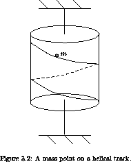
a. What are the degrees of freedom of this system? Pick and describe a convenient set of generalized coordinates for this problem. Write a Lagrangian to describe the dynamical behavior. It may help to know that the moment of inertia of a cylinder around its axis is (1/2)MR2. You may find it easier to do the algebra if various constants are combined and represented as single symbols.
b. Make a Hamiltonian for the system. Write Hamilton's equations for the system. Are there any conserved quantities?
c. If we release the mass point at time t = 0 at the top of the track with zero initial speed and let it slide down, what is the motion of the system?
Exercise 3.7. An ellipsoidal bowl
Consider a point particle of mass m constrained to move in a bowl
and acted upon by a uniform gravitational acceleration g. The bowl
is ellipsoidal, with height z = a x2 + b y2. Make a Hamiltonian
for this system. Can you make any immediate deductions
about this system?
The previous two derivations of Hamilton's equations have made use of the Lagrange equations. Hamilton's equations can also be derived directly from the action principle.
The action is the integral of the Lagrangian along a path:

The action is stationary with respect to variations of the path that preserve the configuration at the endpoints (for Lagrangians that are functions of time, coordinates, and velocities).
We can rewrite the integrand in terms of the Hamiltonian

with p(t) = 2 L(t, q(t), Dq(t)). The Legendre
transformation construction gives

which is one of Hamilton's equations, the one that does not depend on the path being a realizable path.
In order to vary the action we need to make the dependences on the path explicit. We introduce

so p(t) =  [q](t)
and14
[q](t)
and14

The integrand of the action integral is then

The variation of the action is
where  [q] is the variation in the momentum.15
Integrating the second term by parts, using
D([q] q) = D([q]) q + [q] D q, we get
[q] is the variation in the momentum.15
Integrating the second term by parts, using
D([q] q) = D([q]) q + [q] D q, we get
The variations are constrained so that q(t1) = q(t2)
= 0, so the integrated part vanishes. The variation of the action
is
As a consequence of equation (3.68), the factor
multiplying [q] is zero. We are left with

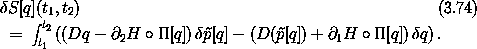
For the variation of the action to be zero for arbitrary variations, except for the endpoint conditions, we must have

Using using p(t) = [q](t), this is

which is the ``dynamical'' Hamilton equation.16
Figure 3.3 shows a summary of the functional
relationship between the Lagrangian and the Hamiltonian descriptions
of a dynamical system. The diagram shows a ``circuit''
interconnecting some ``devices'' with ``wires.'' The devices
represent the mathematical functions that relate the quantities on
their terminals. The wires represent identifications of the
quantities on the terminals that they connect. For example, there is
a box that represents the Lagrangian function. Given values t, q,
and  , the value of the Lagrangian L(t, q, ) is on the
terminal labeled L, which is wired to an addend terminal of an
adder. Other terminals of the Lagrangian carry the
values of the partial derivatives of the Lagrangian function.
, the value of the Lagrangian L(t, q, ) is on the
terminal labeled L, which is wired to an addend terminal of an
adder. Other terminals of the Lagrangian carry the
values of the partial derivatives of the Lagrangian function.
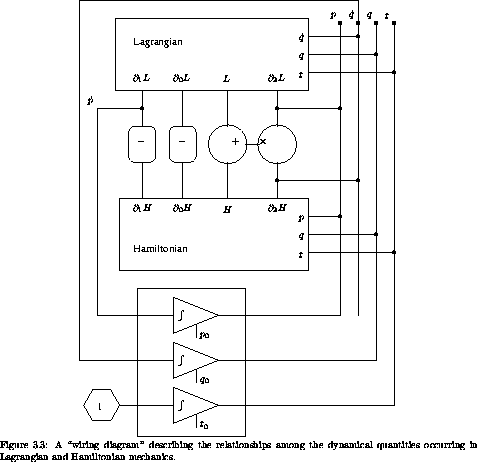
The upper part of the diagram summarizes the relationship of the
Hamiltonian to the Lagrangian. For example, the sum of the values on
the terminals L of the Lagrangian and H of the Hamiltonian is the
product of the value on the terminal of the Lagrangian and
the value on the p terminal of the Hamiltonian. This is the active
part of the Legendre transform. The passive variables are related by
the corresponding partial derivatives being negations of each other.
In the lower part of the diagram the equations of motion are indicated
by the presence of the integrators, relating the dynamical quantities
to their time derivatives.
One can use this diagram to help understand the underlying unity of
the Lagrangian and Hamiltonian formulations of mechanics. Lagrange's
equations are just the connection of the  wire to the
1 L terminal of the Lagrangian device. One of Hamilton's
equations is just the connection of the wire (through the
negation device) to the 1 H terminal of the Hamiltonian
device. The other is just the connection of the wire to the
2 H terminal of the Hamiltonian device. We see that the
two formulations are consistent. One does not have to abandon any
part of the Lagrangian formulation to use the Hamiltonian formulation:
there are deductions that can be made using both simultaneously.
wire to the
1 L terminal of the Lagrangian device. One of Hamilton's
equations is just the connection of the wire (through the
negation device) to the 1 H terminal of the Hamiltonian
device. The other is just the connection of the wire to the
2 H terminal of the Hamiltonian device. We see that the
two formulations are consistent. One does not have to abandon any
part of the Lagrangian formulation to use the Hamiltonian formulation:
there are deductions that can be made using both simultaneously.
1 Here we restrict our attention to Lagrangians that depend only on the time, the coordinates, and the velocities.
2 Here we are using mnemonic names t, q, p for formal parameters of the function being defined. We could have used names like a, b, c as above, but this would have made the argument harder to read.
3 P = I2.
4 The overall minus sign in the definition of the Hamiltonian is traditional.
5 In traditional notation, Hamilton's equations are written:
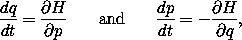
or as separate equations for each component:
6 Traditionally, the Hamiltonian is written

This way of writing the Hamiltonian confuses the values of
functions with the functions that generate them: both and
L must be reexpressed as functions of the time, coordinates, and
momenta.
7 In the construction of the Lagrangian state derivative from the
Lagrange equations we must solve for the highest-order derivative.
The solution process requires the inversion of 2
2 L. In the construction of Hamilton's equations, the
construction of from the momentum state function
2 L requires the inverse of the same structure.
If the Lagrangian formulation has singularities, they
cannot be avoided by going to the Hamiltonian formulation.
8 The term phase space was introduced by Josiah Willard Gibbs in his formulation of statistical mechanics. The Hamiltonian plays a fundamental role in the Boltzmann-Gibbs formulation of statistical mechanics and in both the Heisenberg and Schrödinger approaches to quantum mechanics.
The momentum p can be viewed as the
coordinate representation of a linear form on
the tangent space. Thus p is a scalar quantity that is
invariant under time-independent coordinate transformations of the configuration
space. The set of
momentum forms comprise an n-dimensional vector space at each point
of the configuration space called the
cotangent space. The collection of all cotangent spaces of a
configuration space forms a space called the cotangent
bundle of the configuration manifold.
9 By default, literal functions map reals to reals; the default type for a literal function is (-> Real Real). Here, the potential energy V takes two real arguments and returns a real.
10 The Legendre transformation is more general than its use in mechanics in that it captures the relationship between conjugate variables in systems as diverse as thermodynamics, circuits, and field theory.
11 This can be done so long as the derivative is not zero.
12 If M is the matrix representation of M, then M = MT.
13 The division operation, denoted by / in the Legendre-transform procedure, is generic over mathematical objects. We interpret the division in the matrix representation as follows: a vector y divided by a matrix M is interpreted as a request to solve the linear system M x = y, where x is the unknown vector.
14 The function [q] is the same as L[q] introduced
previously. Indeed, the Lagrangian is needed to define momentum in
every case, but we are suppressing the dependency here because it
does not matter in this argument.
15 The variation of the momentum [q] need not be
further expanded in this argument because it turns out that the factor
multiplying it is zero. However, it is handy to see how it is related
to the variations in the coordinate path q:

16 It is sometimes asserted that the momenta have a different
status in the Lagrangian and Hamiltonian formulations: that in the
Hamiltonian framework the momenta are ``independent'' of the
coordinates. From this it is argued that the
variations q and p are arbitrary and independent,
therefore implying that the factor multiplying each of
them in the action integral (3.74) must
independently be zero, apparently deriving both of Hamilton's
equations. The argument is fallacious: we can write p in
terms of q (see
footnote 15).