Lagrange's equations are ordinary differential equations that the path must satisfy. They can be used to test if a proposed path is a realizable path of the system. However, we can also use them to develop a path, starting with initial conditions.
The state of a system is defined to be the information that must be specified for the subsequent evolution to be determined. Remember our juggler: he or she must throw the pin in a certain way for it to execute the desired motion. The juggler has control of the initial position and orientation of the pin, and the initial velocity and spin of the pin. Our experience with juggling and similar systems suggests that the initial configuration and the rate of change of the configuration are sufficient to determine the subsequent motion. Other systems may require higher derivatives of the configuration.
For Lagrangians that are written in terms of a set of generalized coordinates and velocities we have shown that Lagrange's equations are second-order ordinary differential equations. If the differential equations can be solved for the highest-order derivatives and if the differential equations satisfy appropriate conditions,73 then there is a unique solution to the initial-value problem: given values of the solution and the lower derivatives of the solution at a particular moment, there is a unique solution function. Given irredundant coordinates the Lagrange equations satisfy these conditions.74 Thus a trajectory is determined by the generalized coordinates and the generalized velocities at any time. This is the information required to specify the dynamical state.
A complete local description of a path consists of the path and all of its derivatives at a moment. The complete local description of a path can be reconstructed from an initial segment of the local tuple, given a prescription for computing higher-order derivatives of the path in terms of lower-order derivatives. The state of the system is specified by that initial segment of the local tuple from which the rest of the complete local description can be deduced. The complete local description gives us the path near that moment. Actually, all we need is a rule for computing the next higher derivative; we can get all the rest from this. Assume that the state of a system is given by the tuple ( t, q, v ). If we are given a prescription for computing the acceleration a = A(t, q, v), then


and so on. So the higher-derivative components of the local tuple are given by functions Dt A, Dt2 A, .... Each of these functions depends on lower-derivative components of the local tuple. All we need to deduce the path from the state is a function that gives the next-higher derivative component of the local description from the state. We use the Lagrange equations to find this function.
First, we expand the Lagrange equations

so that the second derivative appears explicitly:

Solving this system for D2q, one obtains the generalized acceleration along a solution path q:

where [  2
2  2 L o
2 L o  ] is a
structure that can be represented by a symmetric square matrix, so we can
compute its inverse.
The function that gives the acceleration is

where  = I2 is the velocity component selector.
That initial segment of the local tuple that specifies the state is called the local state tuple, or, more simply, the state tuple.
We can express the function that gives the acceleration as a function of the state tuple as the following procedure. It takes a procedure that computes the Lagrangian, and returns a procedure that takes a state tuple as its argument and returns the acceleration.75
(define (Lagrangian->acceleration L)
(let ((P ((partial 2) L))
(F ((partial 1) L)))
(/ (- F
(+ ((partial 0) P)
(* ((partial 1) P) velocity)))
((partial 2) P))))
Once we have a way of computing the acceleration from the coordinates and the velocities, we can give a prescription for computing the derivative of the state as a function of the state. For the state ( t, q(t), Dq(t) ) at the moment t the derivative of the state is ( 1, Dq(t), D2q(t) ) = ( 1, Dq(t), A(t, q(t), Dq(t)) ). The procedure Lagrangian->state-derivative takes a Lagrangian and returns a procedure that takes a state and returns the derivative of the state:
(define (Lagrangian->state-derivative L)
(let ((acceleration (Lagrangian->acceleration L)))
(lambda (state)
(up 1
(velocity state)
(acceleration state)))))
We represent a state by an up-tuple of the components of that initial segment of the local tuple that determine the state.
For example, the parametric state derivative for a harmonic oscillator is
(define (harmonic-state-derivative m k)
(Lagrangian->state-derivative (L-harmonic m k)))
(print-expression
((harmonic-state-derivative 'm 'k)
(up 't (up 'x 'y) (up 'v_x 'v_y))))
(up 1 (up v_x v_y) (up (/ (* -1 k x) m) (/ (* -1 k y) m)))
The Lagrange equations are a second-order system of differential equations that constrain realizable paths q. We can use the state derivative to express the Lagrange equations as a first-order system of differential equations that constrain realizable coordinate paths q and velocity paths v:
(define ((Lagrange-equations-first-order L) q v)
(let ((state-path (qv->state-path q v)))
(- (D state-path)
(compose (Lagrangian->state-derivative L)
state-path))))
(define ((qv->state-path q v) t)
(up t (q t) (v t)))
For example, we can find the first-order form of the equations of motion of a two-dimensional harmonic oscillator:
(show-expression
(((Lagrange-equations-first-order (L-harmonic 'm 'k))
(up (literal-function 'x)
(literal-function 'y))
(up (literal-function 'v_x)
(literal-function 'v_y)))
't))

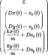
The zero in the first element of the structure of the Lagrange equations residuals is just the tautology that time advances uniformly: the time function is just the identity, so its derivative is one and the residual is zero. The equations in the second element constrain the velocity path to be the derivative of the coordinate path. The equations in the third element give the rate of change of the velocity in terms of the applied forces.

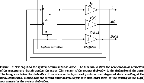
A set of first-order ordinary differential equations that give the state derivative in terms of the state can be integrated to find the state path that emanates from a given initial state. Numerical integrators find approximate solutions of such differential equations by a process illustrated in figure 1.6. The state derivative produced by Lagrangian->state-derivative can be used by a package that numerically integrates systems of first-order ordinary differential equations.
The procedure state-advancer can be used to find the state of a system at a specified time, given an initial state, which includes the initial time, and a parametric state-derivative procedure.76 For example, to advance the state of a two-dimensional harmonic oscillator we write77
(print-expression
((state-advancer harmonic-state-derivative 2 1)
(up 0 (up 1 2) (up 3 4))
10
1.e-12))
(up 10.
(up 3.712791664584467 5.420620823651575)
(up 1.6148030925459906 1.8189103724750977))
The arguments to state-advancer are a parametric state derivative, harmonic-state-derivative, and the state-derivative parameters (mass 2 and spring constant 1). A procedure is returned that takes an initial state, (up 0 (up 1 2) (up 3 4)); a target time, 10; and a relative error tolerance, 1.e-12. The output is an approximation to the state at the specified final time.
Consider the driven pendulum described
above with a periodic drive. We choose ys(t) = a cos  t.
t.
(define ((periodic-drive amplitude frequency phase) t)
(* amplitude (cos (+ (* frequency t) phase))))
(define (L-periodically-driven-pendulum m l g a omega)
(let ((ys (periodic-drive a omega 0)))
(L-pend m l g ys)))
Lagrange's equation for this system is
(show-expression
(((Lagrange-equations
(L-periodically-driven-pendulum 'm 'l 'g 'a 'omega))
(literal-function 'theta))
't))

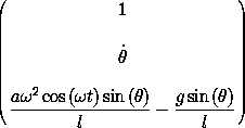
The parametric state derivative for the periodically driven pendulum is
(define (pend-state-derivative m l g a omega)
(Lagrangian->state-derivative
(L-periodically-driven-pendulum m l g a omega)))
(show-expression
((pend-state-derivative 'm 'l 'g 'a 'omega)
(up 't 'theta 'thetadot)))

To examine the evolution of the driven pendulum we need a mechanism that evolves a system for some interval while monitoring aspects of the system as it evolves. The procedure evolve provides this service, using state-advancer repeatedly to advance the state to the required moments. The procedure evolve takes a parametric state derivative and its parameters and returns a procedure that evolves the system from a specified initial state to a number of other times, monitoring some aspect of the state at those times. To generate a plot of the angle versus time we make a monitor procedure that generates the plot as the evolution proceeds:78
(define ((monitor-theta win) state)
(let ((theta ((principal-value :pi) (coordinate state))))
(plot-point win (time state) theta)))
(define plot-win (frame 0. 100. :-pi :pi))
((evolve pend-state-derivative
1.0 ;m=1kg
1.0 ;l=1m
9.8 ;g=9.8m/s2
0.1 ;a=1/10 m
(* 2.0 (sqrt 9.8)) ) ;omega
(up 0.0 ;t0=0
1. ;theta0=1 radian
0.) ;thetadot0=0 radians/s
(monitor-theta plot-win)
0.01 ;step between plotted points
100.0 ;final time
1.0e-13) ;local error tolerance

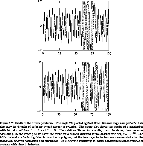
Figure 1.7 shows the angle  versus time for a couple of orbits for the driven pendulum. The
initial conditions for the two runs are the same except that in one
the bob is given a tiny velocity equal to 10-10 m/s, about one
atom width per second. The initial segments of the two orbits are
indistinguishable. After about 75 seconds the two orbits diverge and
become completely different. This extreme sensitivity to tiny changes
in initial conditions is characteristic of what is called chaotic
behavior. Later, we will investigate this example further, using
other tools such as Lyapunov exponents, phase space, and Poincaré
sections.
73 For example, the Lipschitz condition is that the rate of change of the derivative is bounded by a constant in an open set around each point of the trajectory. See [25] for a good treatment of the Lipschitz condition.
74 If the coordinates are redundant we cannot, in general, solve for the highest-order derivative. However, since we can transform to irredundant coordinates, since we can solve the initial-value problem in the irredundant coordinates, and since we can construct the redundant coordinates from the irredundant coordinates, we can in general solve the initial-value problem for redundant coordinates. The only hitch is that we cannot specify arbitrary initial conditions: the initial conditions must be consistent with the constraints.
75 In Scmutils, division by a structure is interpreted as multiplication on the left by the inverse structure.
76 The Scmutils system provides a stable of numerical integration routines that can be accessed through this interface. These include quality-controlled Runge-Kutta and Bulirsch-Stoer. The default integration method is Bulirsch-Stoer.
77 The procedure state-advancer automatically compiles state-derivative procedures the first time they are encountered. The first time a new state derivative is used there is a delay while compilation occurs.
78 The results are plotted in a plot window created by the procedure frame with arguments xmin, xmax, ymin, and ymax that specify the limits of the plotting area. Points are added to the plot with the procedure plot-point that takes a plot window and the abscissa and ordinate of the point to be plotted.
The procedure principal-value is used to reduce an angle to a
standard interval. The argument to principal-value is the
point at which the circle is to be cut. Thus (principal-value :pi)
is a procedure that reduces an angle  to the interval -
  <
<  <
<  .
.