2
Rigid Bodies
The polhode rolls without slipping on the herpolhode lying in the invariable plane.
Herbert Goldstein, Classical Mechanics [20], footnote, p. 207.
The motion of rigid bodies presents many surprising phenomena.
Consider the motion of a top. A top is usually thought of as an axisymmetric body, subject to gravity, with a point on the axis of symmetry that is fixed in space. The top is spun and in general executes some complicated motion. We observe that the top usually settles down into an unusual motion in which the axis of the top slowly precesses about the vertical, apparently moving perpendicular to the direction in which gravity is attempting to accelerate it.
Consider the motion of a book thrown into the air.1 Books have three main axes. If we idealize a book as a brick with rectangular faces, the three axes are the lines through the centers of opposite faces. Try spinning the book about each axis. The motion of the book spun about the longest and the shortest axis is a simple regular rotation, perhaps with a little wobble depending on how carefully it is thrown. The motion of the book spun about the intermediate axis is qualitatively different: however carefully the book is spun about the intermediate axis, it tumbles.
The rotation of the Moon is peculiar in that the Moon always presents the same face to the Earth, indicating that the rotational period and the orbit period are the same. Considering that the orbit of the Moon is constantly changing because of interactions with the Sun and other planets, and therefore its orbital period is constantly undergoing small variations, we might expect that the face of the Moon that we see would slowly change, but it does not. What is special about the face that is presented to us?
A rigid body may be thought of as a large number of constituent particles with rigid constraints among them. Thus the dynamical principles governing the motion of rigid bodies are the same as those governing the motion of any other system of particles with rigid constraints. What is new here is that the number of constituent particles is very large and we need to develop new tools to handle them effectively.
We have found that a Lagrangian for a system with rigid constraints can be written as the difference of the kinetic and potential energies. The kinetic and potential energies are naturally expressed in terms of the positions and velocities of the constituent particles. To write the Lagrangian in terms of the generalized coordinates and velocities we must specify functions that relate the generalized coordinates to the positions of the constituent particles. In the systems with rigid constraints considered up to now these functions were explicitly given for each of the constituent particles and individually included in the derivation of the Lagrangian. For a rigid body, however, there are too many consituent particles to handle each one of them in this way. We need to find means of expressing the kinetic and potential energies of rigid bodies in terms of the generalized coordinates and velocities, without going through the particle-by-particle details.
The strategy is to first rewrite the kinetic and potential energies in terms of quantities that characterize essential aspects of the distribution of mass in the body and the state of motion of the body. Only later do we introduce generalized coordinates. For the kinetic energy, it turns out a small number of parameters completely specify the state of motion and the relevant aspects of the distribution of mass in the body. For the potential energy, we find that for some specific problems the potential energy can be represented with a small number of parameters, but in general we have to make approximations to obtain a representation with a manageable number of parameters.
2.1 Rotational Kinetic Energy
We consider a rigid body to be made up of a large number of constituent particles with mass mα, position
It turns out that the kinetic energy of a rigid body can be separated into two pieces: a kinetic energy of translation and a kinetic energy of rotation. Let’s see how this comes about.
The configuration of a rigid body is fully specified given the location of any point in the body and the orientation of the body. This suggests that it would be useful to decompose the position vectors for the constituent particles as the sum of the vector
Along paths, the velocities are related by
So in terms of
If we select the reference position in the body to be its center of mass,
where
So along paths the relative velocities satisfy
The kinetic energy is then
The kinetic energy is the sum of the kinetic energy of the motion of the total mass at the center of mass
and the kinetic energy of rotation about the center of mass
Written in terms of appropriate generalized coordinates, the kinetic energy is a Lagrangian for a free rigid body. If we choose generalized coordinates so that the center of mass position is entirely specified by some of them and the orientation is entirely specified by others, then the Lagrange equations for a free rigid body will decouple into two groups of equations, one concerned with the motion of the center of mass and one concerned with the orientation.
Such a separation might occur in other problems, such as a rigid body moving in a uniform gravitational field, but in general, potential energies cannot be separated as the kinetic energy separates. So the motion of the center of mass and the rotational motion are usually coupled through the potential. Even in these cases, it is usually an advantage to choose generalized coordinates that separately specify the position of the center of mass and the orientation.
2.2 Kinematics of Rotation
The motion of a rigid body about a center of rotation, a reference position that is fixed with respect to the body, is characterized at each moment by a rotation axis and a rate of rotation. Let’s elaborate.
We can get from any orientation of a body to any other orientation of the body by a rotation of the body. That this is true is called Euler’s theorem on rotations about a point.2 We know that rotations have the property that they do not commute: the composition of successive rotations in general depends on the order of operation. Rotating a book about the
We can specify the orientation of a body by specifying the rotation that takes the body to its actual orientation from some reference orientation. As the body moves, the rotation that does this changes.
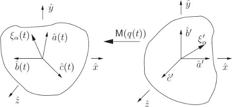
Let q be the coordinate path that we will use to describe the motion of the body. Let
The constituent vectors
To compute the kinetic energy we will accumulate the contributions from all of the constituent mass elements. So we need the velocities of the constituents. The positions of the constituent particles, at a given time t, are
where
Using equation (2.12), we can write
So we have a time-varying linear differential equation that describes the motion of the constituents. Let’s look at the multiplier DM(t)(M(t))−1. Since M(t) is a rotation its matrix representation is an orthogonal matrix M(t), with the property
So
We can conclude that
Let u have components (x, y, z). Every 3 × 3 antisymmetric matrix is of the following form:
Multiplication by this matrix can be interpreted as the operation of cross product with the vector
The inverse of the function
We can interpret multiplication by
In terms of the angular velocity vector, the differential equations for the motion of the constituents (see equation 2.14) are
If the angular velocity vector for a body is
The components ω′ of the angular velocity vector on the body axes are
The relationship of the angular velocity vector to the path is a kinematic relationship; it is valid for any path. Thus we can abstract it to obtain the components of the angular velocity at a moment given the configuration and velocity at that moment.
Implementation of angular velocity functions
The following procedure gives the components of the angular velocity as a function of time along the path:
(define (((M-of-q->omega-of-t M-of-q) q) t)
(define M-on-path (compose M-of-q q))
(define (omega-cross t)
(* ((D M-on-path) t)
(transpose (M-on-path t))))
(antisymmetric->column-matrix (omega-cross t)))
The procedure omega-cross produces the matrix representation of
The components of the angular velocity vector on a basis fixed in the body, as a function of time, along the path are
(define (((M-of-q->omega-body-of-t M-of-q) q) t)
(* (transpose (M-of-q (q t)))
(((M-of-q->omega-of-t M-of-q) q) t)))
We can get the procedures of local state that give the angular velocity components by abstracting these procedures along arbitrary paths that have given coordinates and velocities. The abstraction of a procedure of a path to a procedure of state is accomplished by Gamma-bar (see section 1.9):
(define (M->omega M-of-q)
(Gamma-bar
(M-of-q->omega-of-t M-of-q)))
(define (M->omega-body M-of-q)
(Gamma-bar
(M-of-q->omega-body-of-t M-of-q)))
These procedures give the angular velocities as a function of state. We will see them in action after we get some M-of-q’s to work with, starting in section 2.7.
2.3 Moments of Inertia
The rotational kinetic energy is the sum of the kinetic energy of each of the constituents of the rigid body. We can rewrite the rotational kinetic energy in terms of the angular velocity vector and certain aggregate quantities determined by the distribution of mass in the rigid body.
Substituting our representation of the relative velocity vectors into the rotational kinetic energy, we obtain
We introduce an arbitrary spatially fixed rectangular coordinate system with origin at the center of rotation and with basis vectors ê0, ê1, and ê2, with the property that ê0 × ê1 = ê2. The components of
with
The nine time-dependent quantities Iij are the components of the inertia tensor with respect to the chosen coordinate system.
Note what a remarkable form the kinetic energy has taken. All we have done is interchange the order of summations, but now the kinetic energy is written as a sum of products of components of the angular velocity vector, which completely specify how the orientation of the body is changing, and the quantity Iij, which depends solely on the distribution of mass in the body relative to the chosen coordinate system.
We will deduce a number of properties of the inertia tensor. First, we find a somewhat simpler expression for it. The components of the vector
where
Note that the inertia tensor has real components and is symmetric: Ijk = Ikj.
We define the moment of inertia about a line by
where
The rotational kinetic energy of a body depends on the distribution of mass of the body solely through the inertia tensor. Remarkably, the inertia tensor involves only second-order moments of the mass distribution with respect to the center of mass. We might have expected the kinetic energy to depend in a complicated way on all the moments of the mass distribution, interwoven in some complicated way with the components of the angular velocity vector, but this is not the case. This fact has a remarkable consequence: for the motion of a free rigid body the detailed shape of the body does not matter. If a book and a banana have the same inertia tensor, that is, the same second-order mass moments, then if they are thrown in the same way the subsequent motion will be the same, however complicated that motion is. The facts that the book has corners and the banana has a stem do not affect the motion except for their contributions to the inertia tensor. In general, the potential energy of an extended body is not so simple and does indeed depend on all moments of the mass distribution, but for the kinetic energy the second moments are all that matter!
Exercise 2.1: Rotational kinetic energy
Show that the rotational kinetic energy can also be written
where I is the moment of inertia about the line through the center of mass with direction
Exercise 2.2: Steiner’s theorem
Let I be the moment of inertia of a body with respect to some given line through the center of mass. Show that the moment of inertia I′ with respect to a second line parallel to the first is
where M is the total mass of the body and R is the distance between the lines.
Exercise 2.3: Some useful moments of inertia
Show that the moments of inertia of the following objects are as given:
a. The moment of inertia of a sphere of uniform density with mass M and radius R about any line through the center is
b. The moment of inertia of a spherical shell with mass M and radius R about any line through the center is
c. The moment of inertia of a cylinder of uniform density with mass M and radius R about the axis of the cylinder is
d. The moment of inertia of a thin rod of uniform density per unit length with mass M and length L about an axis perpendicular to the rod through the center of mass is
Exercise 2.4: Jupiter
a. The density of a planet increases toward the center. Provide an argument that the moment of inertia of a planet is less than that of a sphere of uniform density of the same mass and radius.
b. The density as a function of radius inside Jupiter is well approximated by
where M is the mass and R is the radius of Jupiter. Find the moment of inertia of Jupiter in terms of M and R.
2.4 Inertia Tensor
The representation of the rotational kinetic energy in terms of the inertia tensor was derived with the help of a rectangular coordinate system with basis vectors êi. There was nothing special about this particular rectangular basis. So, the kinetic energy must have the same form in any rectangular coordinate system. We can use this fact to derive how the inertia tensor changes if the body or the coordinate system is rotated.
Let’s talk a bit about active and passive rotations. The rotation of the vector
Alternatively, we can rotate the coordinate system by rotating the basis vectors, but leave other vectors that might be represented in terms of them unchanged. If a vector is unchanged but the basis vectors are rotated, then the components of the vector on the rotated basis vectors are not the same as the components on the original basis vectors. Denote the rotated basis vectors by
With respect to the rectangular basis êi the rotational kinetic energy is written
In terms of matrix representations, the kinetic energy is
where ω is the column of components representing
where R is the matrix representation of R. The kinetic energy is
However, if we had started with the basis
where the components are taken with respect to the
Thus the inertia matrix transforms by a similarity transformation.6
2.5 Principal Moments of Inertia
We can use the transformation properties of the inertia tensor (2.35) to show that there are special rectangular coordinate systems for which the inertia tensor I′ is diagonal, that is,
We can examine pieces of this matrix equation by multiplying on the right by a trivial column vector that picks out a particular column. So we multiply on the right by the column matrix representation ei of each of the coordinate unit vectors êi. These column matrices have a one in the ith row and zeros otherwise. Using
On the other hand, the matrix I′ is diagonal, so
So, from equations (2.37) and (2.38), we have
which we recognize as an equation for the eigenvalue
From
If a matrix is real and symmetric then the eigenvalues are real. Furthermore, if the eigenvalues are distinct then the eigenvectors are orthogonal. However, if the eigenvalues are not distinct then the directions of the eigenvectors for the degenerate eigenvalues are not uniquely determined—we have the freedom to choose particular
The eigenvectors and eigenvalues are determined by the requirement that the inertia tensor be diagonal with respect to the rotated coordinate system. Thus the rotated coordinate system has a special orientation with respect to the body. The basis vectors
For convenience, we often label the principal moments of inertia according to their size: A ≤ B ≤ C, with principal axis unit vectors â,
Let x represent the matrix of components of a vector
The components of a vector on the principal axis basis are sometimes called the body components of the vector.
If we choose the reference orientation of the body so that the principal axes are aligned with the spatial axes
Now let’s rewrite the kinetic energy in terms of the principal moments of inertia. If we choose our rectangular coordinate system so that it coincides with the principal axes then the calculation is simple. Let the components of the angular velocity vector on the principal axes be (ωa, ωb, ωc). Then, keeping in mind that the inertia tensor is diagonal with respect to the principal axis basis, the kinetic energy is just
Or as a program:
(define ((T-body A B C) omega-body)
(* 1/2
(+ (* A (square (ref omega-body 0)))
(* B (square (ref omega-body 1)))
(* C (square (ref omega-body 2))))))
Exercise 2.5: A constraint on the moments of inertia
Show that the sum of any two of the moments of inertia is greater than or equal to the third moment of inertia. You may assume the moments of inertia are with respect to orthogonal axes.
Exercise 2.6: Principal moments of inertia
For each of the configurations described below find the principal moments of inertia with respect to the center of mass, and find the corresponding principal axes.
a. A regular tetrahedron consisting of four equal point masses tied together with rigid massless wire.
b. A cube of uniform density.
c. Five equal point masses rigidly connected by massless stuff. The point masses are at the rectangular coordinates
(−1, 0, 0), (1, 0, 0), (1, 1, 0), (0, 0, 0), (0, 0, 1).
Exercise 2.7: This book
Measure this book. You will admit that it is pretty dense. Don’t worry, you will get to throw it later. Show that the principal axes are the lines connecting the centers of opposite faces of the idealized brick approximating the book. Compute the corresponding principal moments of inertia.
2.6 Vector Angular Momentum
The vector angular momentum of a particle is the cross product of its position vector and its linear momentum vector. For a rigid body the vector angular momentum is the sum of the vector angular momentum of each of the constituents. Here we find an expression for the vector angular momentum of a rigid body in terms of the inertia tensor and the angular velocity vector.
The vector angular momentum of a rigid body is
where
with velocities
Substituting, the angular momentum is
Multiplying out the product, and using the fact that
The angular momentum of the center of mass is
and the rotational angular momentum is
Using
We can also reexpress the rotational angular momentum in terms of the angular velocity vector and the inertia tensor, as we did for the kinetic energy. In terms of components with respect to the basis {ê0, ê1, ê2}, this is
where Ijk are the components of the inertia tensor (2.24). The angular momentum and the kinetic energy are expressed in terms of the same inertia tensor.
With respect to the principal-axis basis, the components of the angular momentum have a particularly simple form:
Since the angular momenta are the partial derivatives of TR (see equation 2.41) with respect to the angular velocities, they must be grouped as a down tuple (in matrix language, a row matrix): L′ = [La, Lb, Lc]. As a program:
(define ((L-body A B C) omega-body)
(down (* A (ref omega-body 0))
(* B (ref omega-body 1))
(* C (ref omega-body 2))))
If M is the matrix representation of the rotation that takes an angular-velocity vector
When working with matrices it is more convenient to work with a column matrix of the angular momentum components, so we introduce
Transposing this result, we see that the angular momentum components must transform as
(define (((L-space M) A B C) omega-body)
(* ((L-body A B C) omega-body)
(transpose M)))
Exercise 2.8: Rotational angular momentum
Verify that expression (2.50) for the components of the rotational angular momentum (2.49) in terms of the inertia tensor is correct.
2.7 Euler Angles
To go further we must finally specify a set of generalized coordinates. We first do this using the traditional Euler angles. Later, we find other ways of describing the orientation of a rigid body.
We are using an intermediate representation of the orientation in terms of the function
We define the Euler angles in terms of simple rotations about the coordinate axes. Let Rx(ψ) be a right-handed rotation about the
for the Euler angles θ, φ, ψ.
The Euler angles can specify any orientation of the body, but the orientation does not always correspond to a unique set of Euler angles. In particular, if θ = 0 then the orientation is dependent only on the sum φ + ψ, so the orientation does not uniquely determine either φ or ψ.
Exercise 2.9: Euler angles
It is not immediately obvious that all orientations can be represented in terms of the Euler angles. To show that the Euler angles are adequate to represent all orientations, solve for the Euler angles that give an arbitrary rotation R. Keep in mind that some orientations do not correspond to a unique representation in terms of Euler angles.
Though the Euler angles allow us to specify all orientations and thus can be used as generalized coordinates, the definition of Euler angles is pretty arbitrary. In fact no reasoning has led us to them. This is reflected in our presentation of them by just saying “here they are.” Euler angles are well suited for some problems, but cumbersome for others.
There are other ways of defining similar sets of angles. For instance, we could also take our generalized coordinates to satisfy
Such alternatives to the Euler angles sometimes come in handy.
Each of the fundamental rotations can be represented as a matrix. The rotation matrix representing a right-handed rotation about the ẑ axis by the angle ψ is
and a right-handed rotation about the x axis by the angle ψ is represented by the matrix
The matrix that represents the rotation that carries the body from its reference orientation to the actual orientation is
The rotation matrices and their product can be constructed by simple programs:
(define (Rz-matrix angle)
(matrix-by-rows
(list |
(cos angle) | (- (sin angle)) | 0) |
(list |
(sin angle) | (cos angle) | 0) |
(list |
0 |
0 |
1))) |
(define (Rx-matrix angle)
(matrix-by-rows
(list |
1 |
0 |
0) |
(list |
0 |
(cos angle) | (- (sin angle))) |
(list |
0 |
(sin angle) | (cos angle)))) |
(define (Euler->M angles)
(let ((theta (ref angles 0))
(phi |
(ref angles 1)) |
(psi |
(ref angles 2))) |
(* (Rz-matrix phi)
(Rx-matrix theta)
(Rz-matrix psi))))
Now that we have a procedure that implements a sample
(show-expression
(((M-of-q->omega-body-of-t Euler->M)
(up (literal-function ’theta)
(literal-function ’phi)
(literal-function ’psi)))
’t))
To construct the kinetic energy we need the procedure of state that gives the body components of the angular velocity vector:
(show-expression
((M->omega-body Euler->M)
(up ’t
(up ’theta ’phi ’psi)
(up ’thetadot ’phidot ’psidot))))
We capture this result as a procedure:
(define (Euler-state->omega-body local)
(let ((q (coordinate local)) (qdot (velocity local)))
(let ((theta (ref q 0))
(psi (ref q 2))
(thetadot (ref qdot 0))
(phidot (ref qdot 1))
(psidot (ref qdot 2)))
(let ((omega-a (+ |
(* thetadot (cos psi)) |
| (* phidot (sin theta) (sin psi)))) | |
(omega-b (+ |
(* -1 thetadot (sin psi)) |
| (* phidot (sin theta) (cos psi)))) | |
(omega-c (+ |
(* phidot (cos theta)) psidot))) |
(up omega-a omega-b omega-c)))))
The kinetic energy can now be written:
(define ((T-body-Euler A B C) local)
((T-body A B C)
(Euler-state->omega-body local)))
We can define procedures to calculate the components of the angular momentum on the principal axes:
(define ((L-body-Euler A B C) local)
((L-body A B C)
(Euler-state->omega-body local)))
We then transform the components of the angular momentum on the principal axes to the components on the fixed basis êi:
(define ((L-space-Euler A B C) local)
(let ((angles (coordinate local)))
(* ((L-body-Euler A B C) local)
(transpose (Euler->M angles)))))
These procedures are local state functions, like Lagrangians.
2.8 Motion of a Free Rigid Body
The kinetic energy, expressed in terms of a suitable set of generalized coordinates, is a Lagrangian for a free rigid body. In section 2.1 we found that the kinetic energy of a rigid body can be written as the sum of the rotational kinetic energy and the translational kinetic energy. If we choose one set of coordinates to specify the position and another set to specify the orientation, the Lagrangian becomes a sum of a translational Lagrangian and a rotational Lagrangian. The Lagrange equations for translational motion are not coupled to the Lagrange equations for the rotational motion. For a free rigid body the translational motion is just that of a free particle: uniform motion. Here we concentrate on the rotational motion of the free rigid body. We can adopt the Euler angles as the coordinates that specify the orientation; the rotational kinetic energy was expressed in terms of Euler angles in the previous section.
Conserved quantities
The Lagrangian for a free rigid body has no explicit time dependence, so we can deduce that the energy, which is just the kinetic energy, is conserved by the motion.
The Lagrangian does not depend on the Euler angle φ, so we can deduce that the momentum conjugate to this coordinate is conserved. An explicit expression for the momentum conjugate to φ is
(define Euler-state
(up ’t
(up ’theta ’phi ’psi)
(up ’thetadot ’phidot ’psidot)))
(show-expression
(ref (((partial 2) (T-body-Euler ’A ’B ’C)) Euler-state)
1))
We know that this complicated quantity is conserved by the motion of the rigid body because of the symmetries of the Lagrangian.
If there are no external torques, then we expect that the vector angular momentum will be conserved. We can verify this using the Lagrangian formulation of the problem. First, we note that Lz is the same as pφ. We can check this by direct calculation:
(- (ref ((L-space-Euler ’A ’B ’C) Euler-state)
2)
(ref (((partial 2) (T-body-Euler ’A ’B ’C)) Euler-state)
1))
0
We know that pφ is conserved because the Lagrangian for the free rigid body did not mention φ, so now we know that Lz is conserved. Since the orientation of the coordinate axes is arbitrary, we know that if any rectangular component is conserved then all of them are. So the vector angular momentum is conserved for the free rigid body.
We could have seen this with the help of Noether’s theorem (see section 1.8.5). There is a continuous family of rotations that can transform any orientation into any other orientation. The orientation of the coordinate axes we used to define the Euler angles is arbitrary, and the kinetic energy (the Lagrangian) is the same for any choice of coordinate system. Thus the situation meets the requirements of Noether’s theorem, which tells us that there is a conserved quantity. In particular, the family of rotations around each coordinate axis gives us conservation of the angular momentum component on that axis. We construct the vector angular momentum by combining these contributions.
Exercise 2.10: Uniformly accelerated rigid body
Show that a rigid body subject to a uniform acceleration rotates as a free rigid body, while the center of mass has a parabolic trajectory.
Exercise 2.11: Conservation of angular momentum
Fill in the details of the argument that Noether’s theorem implies that vector angular momentum is conserved by the motion of the free rigid body.
2.8.1 Computing the Motion of Free Rigid Bodies
Lagrange’s equations for the motion of a free rigid body in terms of Euler angles are quite disgusting, so we will not show them here. However, we will use the Lagrange equations to explore the motion of the free rigid body.
Before doing this it is worth noting that the equations of motion in Euler angles are singular for some configurations, because for these configurations the Euler angles are not uniquely defined. If we set θ = 0 then an orientation does not correspond to a unique value of φ and ψ; only their sum determines the orientation.
The singularity arises in the explicit Lagrange equations when we attempt to solve for the second derivative of the generalized coordinates in terms of the generalized coordinates and the generalized velocities (see section 1.7). The isolation of the second derivative requires multiplying by the inverse of ∂2∂2L. The determinant of this quantity becomes zero when the Euler angle θ is zero:
(show-expression
(determinant
(((square (partial 2)) (T-body-Euler ’A ’B ’C))
Euler-state)))
So when θ is zero, we cannot solve for the second derivatives. When θ is small, the Euler angles can move very rapidly, and thus may be difficult to compute reliably. Of course, the motion of the rigid body is perfectly well behaved for any orientation. This is a problem of the representation of that motion in Euler angles; it is a “coordinate singularity.”
One solution to this problem is to use another set of Euler-like coordinates for which Lagrange’s equations have singularities for different orientations, such as those defined in equation (2.54). So if as the calculation proceeds the trajectory comes close to a singularity in one set of coordinates, we can switch coordinate systems and use another set for a while until the trajectory encounters another singularity. This solves the problem, but it is cumbersome. For the moment we will ignore this problem and compute some trajectories, being careful to limit our attention to trajectories that avoid the singularities.
We will compute some trajectories by numerical integration and check our integration process by seeing how well energy and angular momentum are conserved. Then, we will investigate the evolution of the components of angular momentum on the principal axis basis. We will discover that we can learn quite a bit about the qualitative behavior of rigid bodies by combining the information we get from the energy and angular momentum.
To develop a trajectory from initial conditions we integrate the Lagrange equations, as we did in chapter 1. The system derivative is obtained from the Lagrangian:
(define (rigid-sysder A B C)
(Lagrangian->state-derivative (T-body-Euler A B C)))
The following program monitors the errors in the energy and in the components of the angular momentum:
(define ((monitor-errors win A B C L0 E0) state)
(let ((t (time state))
(L ((L-space-Euler A B C) state))
(E ((T-body-Euler A B C) state)))
(plot-point win t (relative-error (ref L 0) (ref L0 0)))
(plot-point win t (relative-error (ref L 1) (ref L0 1)))
(plot-point win t (relative-error (ref L 2) (ref L0 2)))
(plot-point win t (relative-error E E0))))
(define (relative-error value reference-value)
(if (zero? reference-value)
(error “Zero reference value -- RELATIVE-ERROR”)
(/ (- value reference-value) reference-value)))
We make a plot window to display the errors:
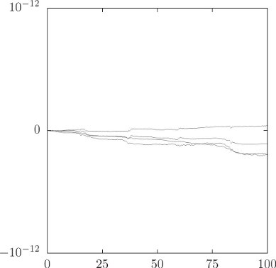
(define win (frame 0.0 100.0 -1.0e-12 1.0e-12))
The default integration method used by the system is Bulirsch–Stoer (bulirsch-stoer), but here we set the integration method to be quality-controlled Runge–Kutta (qcrk4), because the error plot is more interesting:
(set-ode-integration-method! ’qcrk4)
We use evolve to investigate the evolution:
| (let ((A 1.0) (B (sqrt 2.0)) (C 2.0) | ; moments of inertia |
(state0 (up 0.0 |
; initial state |
(up 1.0 0.0 0.0)
(up 0.1 0.1 0.1))))
(let ((L0 ((L-space-Euler A B C) state0))
(E0 ((T-body-Euler A B C) state0)))
((evolve rigid-sysder A B C)
state0
(monitor-errors win A B C L0 E0)
0.1 |
; step between plotted points |
100.0 |
; final time |
1.0e-12))) |
; max local truncation error |
The plot that is developed of the relative errors in the components of the angular momenta and the energy (see figure 2.2) shows that we have been successful in controlling the error in the conserved quantities. This should give us some confidence in the trajectory that is evolved.
2.8.2 Qualitative Features of Free Rigid Body Motion
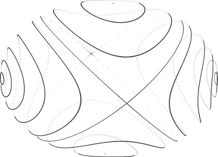
The evolution of the components of the angular momentum on the principal axes has a remarkable property. For almost every initial condition the body components of the angular momentum periodically trace a simple closed curve.
We can see this by investigating a number of trajectories and plotting the components of angular momentum of the body on the principal axes (see figure 2.3). To make this figure a number of trajectories of equal energy were computed. The three-dimensional space of body components is projected onto a two-dimensional plane for display. Points on the back of this projection of the ellipsoid of constant energy are plotted with lower density than points on the front of the ellipsoid. For most initial conditions we find a one-dimensional simple closed curve. Some trajectories on the front side appear to cross trajectories on the back side, but this is an artifact of projection. There is also a family of trajectories that appear to intersect in two points, one on the front side and one on the back side. The curve that is the union of these trajectories is called a separatrix; it separates different types of motion.
What is going on? The state space for a free rigid body is six-dimensional: the three Euler angles and their time derivatives. We know four constants of the motion—the three spatial components of the angular momentum, Lx, Ly, and Lz, and the energy, E. Thus, the motion is restricted to a two-dimensional region of the state space.8 Our experiment shows that the components of the angular momentum trace one-dimensional closed curves in the angular-momentum subspace, so there is something more going on here.
The total angular momentum is conserved if all of the components are, so we also have the constant
The spatial components of the angular momentum do not change, but of course the projections of the angular momentum onto the principal axes do change because the axes move as the body moves. However, the magnitude of the angular momentum vector is the same whether it is computed from components on the fixed basis or components on the principal axis basis. So, the combination
is conserved.
Using the expressions (2.51) for the components of the angular momentum in terms of the components of the angular velocity vector on the principal axes, the kinetic energy (2.41) can be rewritten in terms of the angular momentum components on the principal axes:
The two conserved quantities (2.59 and 2.60) provide constraints on how the components of the angular momentum vector on the principal axes can change. We recognize the conservation of angular momentum constraint (2.59) as the equation of a sphere, and the conservation of kinetic energy constraint (2.60) as the equation for a triaxial ellipsoid. For every trajectory both constraints are satisfied, so the components of the angular momentum move on the intersection of these two surfaces, the energy ellipsoid and the angular momentum sphere. The intersection of an ellipsoid and a sphere with the same center is typically two closed curves, so an orbit is confined to one of these curves. This sheds light on the puzzle posed at the beginning of this section.
Because of our ordering A ≤ B ≤ C, the longest axis of this triaxial ellipsoid coincides with the ĉ direction (all the angular momentum is along the axis of largest principal moment of inertia) and the shortest axis of the energy ellipsoid coincides with the â axis (all the angular momentum is along the smallest moment of inertia). Without actually solving the Lagrange equations, we have found strong constraints on the evolution of the components of the angular momentum on the principal axes.
To determine how the system evolves along these intersection curves we have to use the equations of motion. We observe that the evolution of the components of the angular momentum on the principal axes depends only on the components of the angular momentum on the principal axes, even though the values of these components are not enough to completely specify the dynamical state. Apparently the dynamics of these components is self-contained, and we will see that it can be described in terms of a set of differential equations whose only dynamical variables are the components of the angular momentum on the principal axes (see section 2.9).
We note that there are two axes for which the intersection curves shrink to a point if we hold the energy constant and vary the magnitude of the angular momentum. If the angular momentum starts at these points, the conserved quantities constrain the angular momentum to stay there. These points are equilibrium points for the body components of the angular momentum. However, they are not equilibrium points for the system as a whole. At these points the body is still rotating even though the body components of the angular momentum are not changing. This kind of equilibrium is called a relative equilibrium. We can also see that if the angular momentum is initially slightly displaced from one of these relative equilibria, then the angular momentum is constrained to stay near it on one of the intersection curves. The angular momentum vector is fixed in space, so the principal axis of the equilibrium point of the body rotates stably about the angular momentum vector.
At the principal axis with intermediate moment of inertia, the
This gives some insight into the mystery of the thrown book mentioned at the beginning of the chapter. If one throws a book so that it is initially rotating about either the axis with the largest moment of inertia or the axis with the smallest moment of inertia (the shortest and longest physical axes, respectively), the book rotates regularly about that axis. However, if the book is thrown so that it is initially rotating about the axis of intermediate moment of inertia (the intermediate physical axis), then it tumbles, however carefully it is thrown. You can try it with this book (but put a rubber band or string around it first).
Before moving on, we can make some further physical deductions. Suppose a freely rotating body is subject to some sort of internal friction that dissipates energy but conserves the angular momentum. For example, real bodies flex as they spin. If the spin axis moves with respect to the body then the flexing changes with time, and this changing distortion converts kinetic energy of rotation into heat. Internal processes do not change the total angular momentum of the system. If we hold the magnitude of the angular momentum fixed but gradually decrease the energy, then the curve of intersection on which the system moves gradually deforms. For a given angular momentum there is a lower limit on the energy: the energy cannot be so low that there are no intersections. For this lowest energy the intersection of the angular momentum sphere and the energy ellipsoid is a pair of points on the axis of maximum moment of inertia. With energy dissipation, a freely rotating physical body eventually ends up with the lowest energy consistent with the given angular momentum, which is rotation about the principal axis with the largest moment of inertia (typically the shortest physical axis).
Thus, we expect that given enough time all freely rotating physical bodies will end up rotating about the axis of largest moment of inertia. You can demonstrate this to your satisfaction by twirling a small bottle containing some viscous fluid, such as correction fluid. What you will find is that, whatever spin you try to put on the bottle, it will reorient itself so that the axis of the largest moment of inertia is aligned with the spin axis. Remarkably, this is very nearly true of almost every body in the solar system for which there is enough information to decide. The deviations from principal axis rotation for the Earth are tiny: the angle between the angular momentum vector and the ĉ axis for the Earth is less than one arc-second.10 In fact, the evidence is that all of the planets, the Moon and all the other natural satellites, and almost all of the asteroids rotate very nearly about the largest moment of inertia. We have deduced that this is to be expected using an elementary argument. There are exceptions. Comets typically do not rotate about the largest moment. As they are heated by the sun, material spews out from localized jets, and the back reaction from these jets changes the rotation state. Among the natural satellites, the only known exception is Saturn’s satellite Hyperion, which is tumbling chaotically. Hyperion is especially out of round and subject to strong gravitational torques from Saturn.
2.9 Euler’s Equations
For a free rigid body we have seen that the components of the angular momentum on the principal axes comprise a self-contained dynamical system: the variation of the principal axis components depends only on the principal axis components. Here we derive equations that govern the evolution of these components.
The starting point for the derivation is the conservation of the vector angular momentum. The components of the angular momentum on the principal axes are11
where ω′ is composed of the components of the angular velocity vector on the principal axes and I′ is the matrix representation of the inertia tensor with respect to the principal axis basis:
The body components of the angular momentum L′ are related to the components L on the fixed rectangular basis êi by
where M is the matrix representation of the rotation that carries the body and all vectors attached to the body from the reference orientation of the body to the actual orientation.
The vector angular momentum is conserved for free rigid-body motion, and so are its components on a fixed rectangular basis. So, along solution paths,
Solving, we find
In terms of ω′ this is
where we have used equation (2.21) to write DM in terms of
for any vector with components v and any rotation with matrix representation R. Using this property of
Euler’s equations give the time derivative of the body components of the angular velocity vector entirely in terms of the angular velocity components and the principal moments of inertia. Let ωa, ωb, and ωc denote the components of the angular velocity vector on the principal axes. Then Euler’s equations can be written as the component equations
Alternatively, we can rewrite Euler’s equations in terms of the components of the angular momentum on the principal axes
These equations confirm that the time derivatives of the components of the angular momentum on the principal axes depend only on the components of the angular momentum on the principal axes.
Euler’s equations are very simple, but they do not completely determine the evolution of a rigid body—they do not give the spatial orientation of the body. However, equation (2.21) and property (2.67) can be used to relate the derivative of the orientation matrix to the body components of the angular velocity vector:
A straightforward method of using these equations is to integrate them componentwise as a set of nine first-order ordinary differential equations, with initial conditions determining the initial configuration matrix. Together with Euler’s equations, which describe how the body components of the angular velocity vector change with time, this system of equations governing the motion of a rigid body is complete. However, the reader will no doubt have noticed that this approach is rather wasteful. The fact that the orientation matrix can be specified with only three parameters has not been taken into account. We should be integrating three equations for the orientation, given ω′, not nine. To accomplish this we once again need to parameterize the configuration matrix.
For example, we can use Euler angles to parameterize the orientation:
We form M by composing
This gives us the desired equation for the orientation. Note that it is singular for θ = 0, as are Lagrange’s equations. So Euler’s equations using Euler angles for the configuration have the same problem as did the Lagrange equations using Euler angles. Again, this is a manifestation of the fact that for θ = 0 the orientation depends only on φ+ψ. The singularity in the equations of motion for θ = 0 does not correspond to anything funny in the motion of the rigid body. A practical solution to the singularity problem is to choose another set of Euler-like angles that have a singularity in a different place, and switch from one to the other when the going gets tough.
Exercise 2.12:
Fill in the details of the derivation of equation (2.73). You may want to use the computer to help with the algebra.
Euler’s equations for forced rigid bodies
Euler’s equations were derived for a free rigid body. In general, we must be able to deal with external forcing. How do we do this? First, we derive expressions for the vector torque. Then we include the vector torque in the Euler equations.
We derive the vector torque in a manner analogous to the derivation of the vector angular momentum. That is, we derive one component and then argue that since the coordinate system is arbitrary, all components have the same form.
Suppose we have a rigid body subject to some potential energy that depends only on time and the configuration. A Lagrangian is L = T − V. If we use the Euler angles as generalized coordinates, the last of the three active Euler rotations that define the orientation is a rotation about the ẑ axis by the angle φ. The Lagrange equation for φ gives13
If we define Tz, the component of the torque about the z axis, to be minus the derivative of the potential energy with respect to the angle of rotation of the body about the z axis,
then we see that
We have already identified the momentum conjugate to φ as one component, Lz, of the vector angular momentum
Since the orientation of the reference rectangular basis vectors is arbitrary, we may choose them any way that we please. Thus if we want any component of the vector torque, we may choose the z-axis so that we can compute it in this way. We can conclude that the vector torque gives the rate of change of the vector angular momentum
Having obtained a general prescription for the vector torque, we address how the vector torque may be included in Euler’s equations. Euler’s equations expressed the fact that the vector angular momentum is conserved. Let’s return to that calculation, but now include a torque with components T arranged as a column matrix:
Carrying out the same steps as before, we find
where the components of the torque on the principal axes are
In terms of ω′ this is
in components,
Note that the torque entered only the equations for the body angular momentum and for the body angular velocity vector. The equations that relate the derivative of the orientation to the angular velocity vector are not modified by the torque. In a sense, Euler’s equations contain the dynamics, and the equations governing the orientation are kinematic. Of course, Lagrange’s equations must be modified by the potential that gives rise to the torques; in this sense Lagrange’s equations contain both dynamics and kinematics.
Exercise 2.13: Bicycle wheel
a. Imagine that you are holding a bicycle wheel by the axle (in both hands) and the wheel is spinning so that the top edge is going away from your face. If you torque the wheel by pushing down with your right hand and pulling up with your left hand the wheel will precess. Which way does it try to turn?
b. A free bicycle wheel rolls on a horizontal surface. If it starts to tilt, the torque from gravity will cause the wheel to turn. Which way will it turn? The reasoning that applied to part a does not directly apply to the rolling bicycle wheel, which is not a holonomic system. However, it is interesting to think about whether the behavior of the two systems is related.
2.10 Axisymmetric Tops
We have all played with a top at one time or another. For the purposes of analysis we will consider an idealized top that does not wander around. Thus, an ideal top is a rotating rigid body, one point of which is fixed in space. Furthermore, the center of mass of the top is not at the fixed point, which is the center of rotation, and there is a uniform gravitational acceleration.
For our top we can take the Lagrangian to be the difference of the kinetic energy and the potential energy. We already know how to write the kinetic energy—what is new here is that we must express the potential energy in terms of the configuration. In the case of a body in a uniform gravitational field this is easy. The potential energy is the sum of “mgh” for all the constituent particles:
where g is the gravitational acceleration, hα =
where the last sum is zero because the center of mass is the origin of
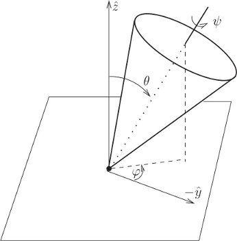
Here we consider an axisymmetric top (see figure 2.4). Such a top has an axis of symmetry of the mass distribution, so the center of mass is on the symmetry axis and the fixed point is also on the axis of symmetry.
In order to write the Lagrangian we need to choose a set of generalized coordinates. If we choose them well we can take advantage of the symmetries of the problem. If the Lagrangian does not depend on a particular coordinate, the conjugate momentum is conserved, and the complexity of the system is reduced.
The axisymmetric top has two apparent symmetries. The fact that the mass distribution is axisymmetric implies that neither the kinetic nor the potential energy is sensitive to the orientation of the top about that symmetry axis. Additionally, the kinetic and potential energy are insensitive to a rotation of the physical system about the vertical axis, because the gravitational field is uniform.
We can take advantage of these symmetries by choosing appropriate coordinates, and we already have a coordinate system that does the job—the Euler angles.14 We choose the reference orientation so that the symmetry axis is vertical. The first Euler angle, ψ, expresses a rotation about the symmetry axis. The next Euler angle, θ, is the tilt of the symmetry axis of the top from the vertical. The third Euler angle, φ, expresses a rotation of the top about the ẑ axis. The symmetries of the problem imply that the first and third Euler angles do not appear in the Lagrangian. As a consequence the momenta conjugate to these angles are conserved quantities. Let’s work out the details.
First, we develop the Lagrangian explicitly. The general form of the kinetic energy about a fixed point is given by equation 2.41. The top is constrained so that it pivots about a fixed point that is not at the center of mass. So the moments of inertia that enter the kinetic energy are the moments of inertia of the top with respect to the pivot point, not with respect to the center of mass. If we know the moments of inertia about the center of mass we can write the moments of inertia about the pivot in terms of them (see exercise 2.2 on Steiner’s theorem). So let’s assume the principal moments of inertia of the top about the pivot are A, B, and C, and A = B because of the symmetry.15 We can use the computer to help us figure out the Lagrangian for this special case:
(show-expression
((T-body-Euler ’A ’A ’C)
(up ’t
(up ’theta ’phi ’psi)
(up ’thetadot ’phidot ’psidot))))
We can rearrange this a bit to get
In terms of Euler angles, the potential energy is
where R is the distance of the center of mass from the pivot. The Lagrangian is L = T − V. We see that the Lagrangian is indeed independent of ψ and φ, as expected.
There is no particular reason to look at the Lagrange equations. We can assign that job to the computer when needed. However, we have already seen that it may be useful to examine the conserved quantities associated with the symmetries.
The energy is conserved, because the Lagrangian has no explicit time dependence. Also, the energy is the sum of the kinetic and potential energy E = T + V, because the kinetic energy is a homogeneous quadratic form in the generalized velocities. The energy is
Two of the generalized coordinates do not appear in the Lagrangian, so there are two conserved momenta. The momentum conjugate to φ is
The momentum conjugate to ψ is
The state of the system at a moment is specified by the tuple
The evolution of the top is described by a four-dimensional subsystem and two auxiliary quadratures.16 This subdivision is a consequence of choosing generalized coordinates that incorporate the symmetries. However, the choice of generalized coordinates that incorporate the symmetries also gives conserved momenta. We can make use of these momenta to simplify the formulation of the problem further. Each conserved quantity can be used to locally eliminate one dimension of the subsystem. In this case the subsystem has four dimensions and there are three conserved quantities, so the system can be completely reduced to quadratures. For the top, this can be done analytically, but we think it is a waste of time to do so. Rather, we are interested in extracting interesting features of the motion. We concentrate on the energy and use the two conserved momenta to eliminate
Along a path θ, where Dθ(t) is substituted for
Let’s get real. Let’s make a top out of an aluminum disk with a steel rod through the center to make the pivot. Measuring the top very carefully, we find that the moment of inertia of the top about the symmetry axis is about 1.32 × 10⁻⁴ kg m2, and the moment of inertia about the pivot point is about 6.96 × 10⁻⁴ kg m2. The combination gM R is about 0.112kg m2 s−2. We spin the top up with an initial angular velocity of
The top initially has
Exercise 2.14: Kinetic energy of the top
The rotational kinetic energy of the top can be written in terms of the principal moments of inertia with respect to the pivot point and the angular velocity vector of rotation with respect to the pivot point. Show that this formulation of the kinetic energy yields the same value that one would obtain by computing the sum of the rotational kinetic energy about its center of mass and the kinetic energy of the motion of the center of mass.
Exercise 2.15: Nutation of the top
a. Carry out the algebra to obtain the energy (2.91) in terms of θ and
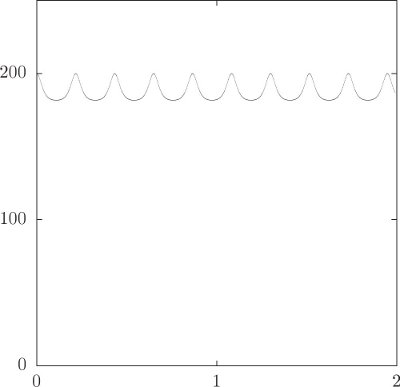
b. Numerically integrate the Lagrange equations for the top to obtain figure 2.5, θ versus time.
c. Note that the energy is a differential equation for
Exercise 2.16: Precession of the top
Consider a top that is rotating so that θ is constant.
a. Using conservation of angular momentum, compute the rate of precession
b. For θ to be at an equilibrium the acceleration D2θ must be zero. Use the Lagrange equation for θ to find the rate of precession
c. Find an approximate expression for the precession rate in the limit that
d. The Newtonian rule is that the rate of change of the angular momentum is the torque. Assume the top is spinning so fast that the angular momentum is nearly the same as the angular momentum of rotation about the symmetry axis. By equating the rate of change of this vector angular momentum to the gravitational torque on the center of mass develop an approximate formula for the precession rate.
e. Numerically integrate the top to check your deductions.
2.11 Spin-Orbit Coupling
The rotation of planets and natural satellites is affected by the gravitational forces from other celestial bodies. As an extended application of the Lagrangian method for forced rigid bodies, we consider the rotation of celestial objects subject to gravitational forces.
We first develop the form of the potential energy for the gravitational interaction of an extended body with an external point mass. With this potential energy and the usual rigid-body kinetic energy we can form Lagrangians that model a number of systems. We will take an initial look at the rotation of the Moon and Mercury; later, after we have developed more tools, we will return to study these systems.
2.11.1 Development of the Potential Energy
The first task is to develop convenient expressions for the gravitational potential energy of the interaction of a rigid body with a distant point mass. A rigid body can be thought of as made of a large number of mass elements, subject to rigid coordinate constraints. We have seen that the kinetic energy of a rigid body is conveniently expressed in terms of the moments of inertia of the body and the angular velocity vector, which in turn can be represented in terms of a suitable set of generalized coordinates. The potential energy can be developed in a similar manner. We first represent the potential energy in terms of moments of the mass distribution and later introduce generalized coordinates as particular parameters of the potential energy.
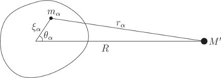
The gravitational potential energy of a point mass and a rigid body (see figure 2.9) is the sum of the potential energy of the point mass with each mass element of the body:
where M′ is the mass of the external point mass, rα is the distance between the point mass and the constituent mass element with index α, mα is the mass of this constituent element, and G is the gravitational constant. Let R be the distance of the center of mass of the rigid body from the point mass. The distance from the center of mass to the constituent with index α is ξα. The distance rα is then given by the law of cosines as
Because this is a three-dimensional body the distance ξα and angle θα do not completely specify the position of the constituent mass element; to do that one must also specify the angle of rotation about the line between the center of mass and the external point mass. But the potential energy does not depend on this angle.
The potential energy is then
This is complete, but we need to find a representation that does not mention each constituent.
Typically, the size of celestial bodies is small compared to the distance between them. We can make use of this to find a more compact representation of the potential energy. If we expand the potential energy in the small ratio ξα/R we find
where Pl is the lth Legendre polynomial.17 Interchanging the order of the summations yields:
Successive terms in this expansion of the potential energy typically decrease very rapidly because celestial bodies are small compared to the distance between them. We can compute an upper bound to the size of these terms by replacing each factor in the sum over α by an upper bound. The Legendre polynomials all have magnitudes less than one for arguments in the range −1 to 1. The distances ξα are all less than some maximum extent of the body ξmax. The sum over mα times these upper bounds is just the total mass M times the upper bounds. Thus
We see that the upper bound on successive terms decreases by a factor ξmax/R. Successive terms may be smaller still. For large bodies the gravitational force is strong enough to overcome the internal material strength of the body, so the body, over time, becomes nearly spherical. Successive terms in the expansion of the potential are measures of the deviation of the mass distribution from a spherical mass distribution. Thus for large bodies the higher-order terms are small because the bodies are nearly spherical.
Consider the first few terms in l. For l = 0 the sum over α just gives the total mass M of the rigid body. For l = 1 the sum over α is zero, as a consequence of choosing the origin of the
where A, B, and C are the principal moments of inertia, and I is the moment of inertia of the rigid body about the line between the center of mass of the body and the external point mass. The moment I depends on the orientation of the rigid body relative to the line between the bodies. The contributions to the potential energy up to l = 2 are then18
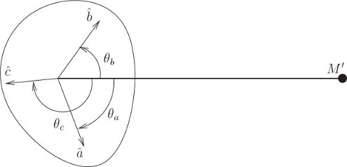
Let ca = cos θa, cb = cos θb, and cc = cos θc be the direction cosines of the angles θa, θb and θc between the principal axes â,
This is a good first approximation to the potential energy of interaction for most situations in the solar system; if we intended to land on the Moon we probably would want to take into account higher-order terms in the expansion.
Exercise 2.17:
a. Fill in the details that show that the sum over constituents in equation (2.97) can be expressed as written in terms of moments of inertia. In particular, show that
and that
b. Show that if the principal moments of inertia of a rigid body are A, B, and C, then the moment of inertia about an axis that goes through the center of mass of the body with angles θa, θb, and θc to the principal axes is
2.11.2 Rotation of the Moon and Hyperion
The approximation to the potential energy that we have derived can be used for a number of different problems. It can be used to investigate the effect of oblateness on the motion of an artificial satellite about the Earth, or to incorporate the effect of planetary oblateness on the evolution of the orbits of natural satellites, such as the Moon or the Galilean satellites of Jupiter. However, as the principal application here, we will use it to investigate the rotational dynamics of natural satellites and planets.
The potential energy depends on the position of the point mass relative to the rigid body and on the orientation of the rigid body. Thus the changing orientation is coupled to the orbital evolution; each affects the other. However, in many situations the effect of the orientation of the body on the evolution of the orbit may be ignored. One way to see this is to look at the relative magnitudes of the two terms in the potential energy (2.99). We already know that the second term is guaranteed to be smaller than the first by a factor of (ξmax/R)2, but often it is much smaller still because the body involved is nearly spherical. For example, the radius of the Moon is about a third the radius of the Earth and the distance to the Moon is about 60 Earth-radii. So the second term is smaller than the first by a factor of order 10−4 due to the size factors. In addition, the Moon is roughly spherical and for any orientation the combination A + B + C − 3I is of order 10−4C. Now C is itself of order
We can learn some important qualitative aspects of the orientation dynamics by studying a simplified model problem. First, we assume that the body is rotating about its largest moment of inertia. This is a natural assumption. Remember that for a free rigid body the loss of energy while conserving angular momentum leads to rotation about the largest moment of inertia. This is observed for most bodies in the solar system. Next, we assume that the spin axis is perpendicular to the orbital motion. This is a good approximation for the rotation of natural satellites, and is a natural consequence of tidal friction—dissipative solid-body tides raised on the satellite by the gravitational interaction with the planet. Finally, for simplicity we take the rigid body to be moving on a fixed elliptic orbit. This may approximate the motion of some physical systems, provided the time scale of the evolution of the orbit is large compared to any time scale associated with the rotational dynamics we are investigating. So we have a nice toy problem, one that has been used to investigate the rotational dynamics of Mercury, the Moon, and other natural satellites. It makes specific predictions concerning the rotation of Phobos, a satellite of Mars, that can be compared with observations. It provides a basic explanation of the fact that Mercury rotates precisely three times for every two orbits it completes, and is the starting point for understanding the chaotic tumbling of Saturn’s satellite Hyperion.
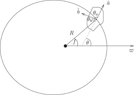
We are assuming that the orbit does not change or precess. The orbit is an ellipse with the point mass at a focus of the ellipse. The angle f (see figure 2.11) measures the position of the rigid body in its orbit relative to the point in the orbit at which the two bodies are closest.19 We assume the orbit is a fixed ellipse, so the angle f and the distance R are periodic functions of time, with period equal to the orbit period. With the spin axis constrained to be perpendicular to the orbit plane, the orientation of the rigid body is specified by a single degree of freedom: the orientation of the body about the spin axis. We specify this orientation by the generalized coordinate θ that measures the angle to the â principal axis from the same line from which we measure f, the line through the point of closest approach.
Having specified the coordinate system, we can work out the details of the kinetic and potential energies, and thus find the Lagrangian. The kinetic energy is
where C is the moment of inertia about the spin axis and the angular velocity of the body about the ĉ axis is
To get an explicit expression for the potential energy, write the direction cosines in terms of θ and f: cos θa = − cos(θ − f), cos θb = sin(θ − f), and cos θc = 0 because the ĉ axis is perpendicular to the orbit plane. The potential energy is then
Since we are assuming that the orbit is given, we need keep only terms that depend on θ. Expanding the squares of the cosine and the sine in terms of the double angles and dropping all the terms that do not depend on θ, we find the potential energy for the orientation20
A Lagrangian for the model spin-orbit coupling problem is then L = T − V :
We introduce the dimensionless “out-of-roundness” parameter
and use the fact that the orbital frequency n and the semimajor axis a satisfy Kepler’s third law, n2a3 = G(M + M′), which is approximately n2a3 = GM′ for a small body in orbit around a much more massive one (M ≪ M′). In terms of ϵ and n the spin-orbit Lagrangian is
This is a problem with one degree of freedom with terms that vary periodically with time.
The Lagrange equations are derived in the usual manner:
The equation of motion is very similar to that of the periodically driven pendulum. The main difference here is that not only is the strength of the acceleration changing periodically, but in the spin-orbit problem the center of attraction is also varying periodically.
We can give a physical interpretation of this equation of motion. It states that the rate of change of the angular momentum is equal to the applied torque. The torque on the body arises because the body is out of round and the gravitational force varies as the inverse square of the distance. Thus the force per unit mass on the near side of the body is a little more than the acceleration of the body as a whole, and the force per unit mass on the far side of the body is a little less than the acceleration of the body as a whole. Thus, relative to the acceleration of the body as a whole, the far side is forced outward while the inner part of the body is forced inward. The net effect is a torque on the body that tries to align the long axis of the body with the line to the external point mass. If θ is a bit larger than f then there is a negative torque, and if θ is a bit smaller than f then there is a positive torque, both of which would align the long axis with the point mass if given a fair chance. The torque arises because of the difference of the inverse R2 force across the body, so the torque is proportional to R−3. There is a torque only if the body is out of round, for otherwise there is no handle to pull on. This is reflected in the factor B − A in the expression for the torque. The potential depends on the mass distribution as described by the moments of inertia, and thus the body has the same dynamics if it is rotated by 180°. The factor of 2 in the argument of sine reflects this symmetry. This torque is called the “gravity gradient torque.”
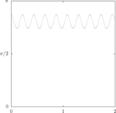
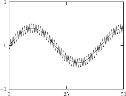
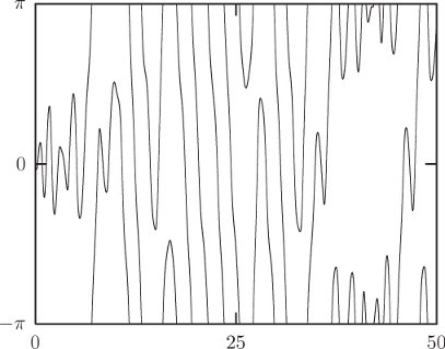
To compute the evolution requires a lot of detailed preparation similar to what has been done for other problems. There are many interesting phenomena to explore. We can take parameters appropriate for the Moon and find that Mr. Moon does not steadily point the same face to the Earth, but instead constantly shakes his head in dismay at what goes on here. If we nudge the Moon a bit, say by hitting it with an asteroid, we find that the long axis oscillates back and forth with respect to the direction that points to the Earth. For the Moon, the orbital eccentricity is currently about 0.05, and the out-of-roundness parameter is about ϵ = 0.026. Figure 2.12 shows the angle θ − f as a function of time for two different values of the “lunar” eccentricity. The plot spans 50 lunar orbits, or a little under four years. This Moon has been kicked by a large asteroid and has initial rotational angular velocity
The oscillation period of the free libration is easily calculated. We see that the eccentricity of the orbit does not substantially affect the period, so we consider the special case of zero eccentricity. In this case R = a, a constant, and f(t) = nt, where n is the orbital frequency.21 The equation of motion becomes
Let φ(t) = θ(t) − nt, and consequently Dφ(t) = Dθ(t) − n, and D2φ = D2θ. Substituting these, the equation governing the evolution of φ is
For small deviations from synchronous rotation (small φ) this is
so we see that the small-amplitude oscillation frequency of φ is nϵ. For the Moon, ϵ is about 0.026, so the period is about 1/0.026 orbit periods or about 40 lunar orbit periods, which is what we observed.
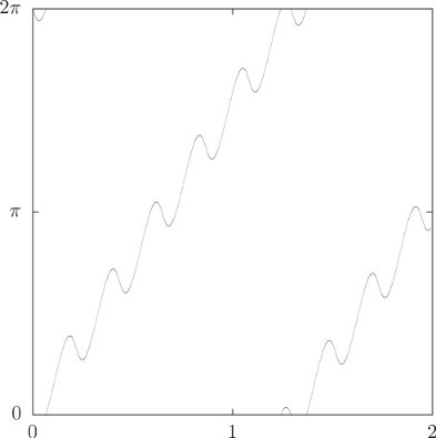
It is perhaps more fun to see what happens if the out-of-roundness parameter is large. After our experience with the driven pendulum it is no surprise that we find abundant chaos in the spin-orbit problem when the system is strongly driven by having large ϵ and significant orbital eccentricity e. There is indeed one body in the solar system that exhibits chaotic rotation—Hyperion, a small satellite of Saturn. Though our toy model is not adequate for a complete account of Hyperion, we can show that it exhibits chaotic behavior for parameters appropriate for Hyperion. We take ϵ = 0.89 and e = 0.1. Figure 2.13 shows θ − f for 50 orbits, starting with θ = 0 and
If we relax our restriction that the spin axis be fixed perpendicular to the orbit, then we find that the Moon maintains this orientation of the spin axis even if nudged a bit, but for Hyperion the spin axis almost immediately falls away from this configuration. The state in which Hyperion on average points one face to Saturn is dynamically unstable to chaotic tumbling. Observations of Hyperion are consistent with the deduction that it is chaotically tumbling.
Exercise 2.18: Precession of the equinox
The Earth spins very nearly about the largest moment of inertia, and the spin axis is tilted by about 23° to the orbit normal. There is a gravity-gradient torque on the Earth from the Sun that causes the spin axis of the Earth to precess. Investigate this precession in the approximation that the orbit of the Earth is circular and the Earth is axisymmetric. Determine the rate of precession in terms of the moments of inertia of the Earth.
2.11.3 Spin-Orbit Resonances
Consider the motion of the Moon in synchronous rotation. We have seen that if we give the Moon a kick so that it is not exactly pointing one face to the Earth, then the face will oscillate back and forth relative to the direction to the Earth. If we give it a really big kick, then instead of oscillating it will spin relative to the direction to the Earth. How do we understand this?
Let’s look again at the equations of motion for the rotation of the Moon when the orbit is circular (equation 2.106):
Changing variables to φ(t) = θ(t) − nt this equation becomes
This equation can be solved; it has an “energy-like” conserved quantity
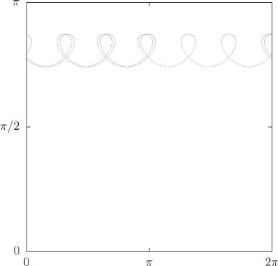
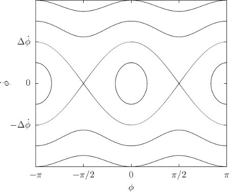
The solutions are just contours of this conserved quantity (see figure 2.14). There are two centers of oscillation corresponding to the two different faces of the Moon that could point towards Earth. There are also trajectories that rotate relative to the Earth. And there are separating trajectories that divided the oscillating trajectories from the circulating trajectories. Where these separating trajectories appear to cross, the system is at an unstable equilibrium. The separating trajectories are asymptotic to the unstable equilibria (a system on that trajectory takes an infinite time to get to the equilibrium point). These asymptotic trajectories are analogous to the trajectories of the simple pendulum that are asymptotic to the vertical.
The extent of the oscillation region can be evaluated with the help of the conserved quantity E. Let’s evaluate it on the separating trajectory:
Equating these and solving, we find the maximum extent of the oscillating region:
So we see that the out-of-roundness parameter ϵ not only gives the frequency of small-amplitude oscillations, but also gives the extent of the oscillation region.
Mercury rotates exactly three times for every two times it goes around the Sun, as discovered by Pettengill and Dyce in 1965, using Arecibo radar. We can understand this spin-orbit resonance using our simple spin-orbit model problem.
Let’s first use qualitative reasoning to understand how the resonance comes about. The spin-orbit equation of motion, equation (2.105), equates the rate of change of the angular momentum to the gravity gradient torque. The torque is proportional to the inverse cube of the distance, so it is largest when the distance is smallest, at pericenter. For the purpose of qualitative reasoning, consider the torque only at pericenter. Suppose Mercury is rotating exactly three times for every two orbits. Then if the long axis of Mercury is pointed at the Sun at one pericenter, it will point the other end of this long axis the next time it passes pericenter (it will have rotated one and a half times). Now, suppose Mercury is rotating a little faster. Then if the long axis is aligned at one pericenter passage, on the next pericenter passage it will have rotated a little too much and the long axis will no longer point to the Sun. In this case θ − f will be positive and there will be a negative torque, slowing down the rotation a bit. Over many orbits the rotation of Mercury is reduced. A similar argument shows that if Mercury is rotating slower than three times for every two orbits, then the torques at succesive pericenter passages will tend to increase the rotation rate. An oscillation ensues.
We can also understand this spin-orbit resonance analytically. The right-hand side of the equation of motion (equation 2.105) has factors that vary periodically with the orbit period:
where both f(t) and R(t) are periodic with period 2π/n. We can expand this as a Fourier series:
where the coefficients Am(e) are functions of the orbital eccentricity e. The coefficients are proportional to e|m−2| and so for small eccentricity we need to consider only a few of them.22 We have
All other terms are of higher order in e. With just the terms of order e or less, the equation of motion becomes
Suppose we are close to the 3:2 Mercury resonance. Then
We can solve this by changing variables to
The equation of motion becomes
This has the “energy-like” conserved quantity
which is very similar to the conserved quantity we found for the zero-eccentricity synchronous rotation case considered earlier; see equation (2.111). Indeed the trajectories are contours of the conserved quantity and look just like those in figure 2.14. Using analogous reasoning we can determine the extent of the oscillation region and find
This gives the approximate range of rotation rate over which Mercury can oscillate stably in the 3:2 resonance.
2.12 Nonsingular Coordinates and Quaternions
The Euler angles provide a convenient way to parameterize the orientation of a rigid body. However, the equations of motion derived for them have singularities. Though we can avoid the singularities by using other Euler-like combinations with different singularities, this kludge is not very satisfying. Let’s brainstorm a bit and see if we can come up with something better.
What does it take to specify an orientation? Perhaps we can take a hint from Euler’s theorem. Recall that Euler’s theorem states that any orientation can be reached with a single rotation. So one idea to specify the orientation of a body is to parameterize this single rotation that does the job. To specify this rotation we need to specify the rotation axis and the amount of rotation. We contrast this with the Euler angles, which specify three successive rotations. These three rotations need not have any relation to the single composite rotation that gives the orientation. Isn’t it curious that the Euler angles make no use of Euler’s theorem?
We can think of several ways of specifying a rotation. One way would be to specify the rotation axis by the latitude and the longitude at which the rotation axis pierces a sphere. The amount of rotation needed to take the body from the reference position could be specified by one more angle. We can predict, though, that this choice of coordinates will have similar problems to those of the Euler angles: if the amount of rotation is zero, then the latitude and longitude of the rotation axis are undefined. So the Lagrange equations for these angles are probably singular. Another idea, without this defect, is to represent the rotation by the rectangular components of an orientation vector
Let θ be the angle of rotation about the axis
where
We can invert this: given a quaternion we can compute the angle and the axis. Let (r, x, y, z) be the components of a quaternion q. We separate the first component (called the real part) and the tuple v = (x, y, z) (called the 3-vector) of the remaining components. The Euclidean norm of the tuple ‖v‖ = | sin(θ/2)|. The first component r = cos(θ/2). So the angle θ = 2 arctan(‖v‖, r) and the axis is v/‖v‖. This process is independent of the scale of the quaternion.
By taking the absolute value of sin(θ/2) we have lost information about the quadrant, but this is not a real problem because the rotation represented by a quaternion is not changed by reversing the sign of all its components: changing the sign of v reverses the axis but does not change the angle; changing the sign of the first component changes the angle θ to 2π − θ, so the actual rotation is unchanged.
Given the four elements of a quaternion, we need to find the corresponding rotation matrix. We can get the angle and axis given a quaternion. We can get a rotation matrix given the angle θ and the axis given by a unit vector
where φ = arccos(
A procedure for making the rotation matrix is:
(define (angle-axis->rotation-matrix theta n)
(let ((nx (ref n 0)) (ny (ref n 1)) (nz (ref n 2)))
(let ((colatitude (acos nz)) (longitude (atan ny nx)))
(* (Rz-matrix longitude)
(Ry-matrix colatitude)
(Rz-matrix theta)
(transpose (Ry-matrix colatitude))
(transpose (Rz-matrix longitude))))))
And a procedure for obtaining the angle and axis of a quaternion is
(define (quaternion->angle-axis q)
(let* ((v (quaternion->3vector q))
(theta (* 2 (atan (euclidean-norm v)
(quaternion->real-part q))))
(axis (/ v (euclidean-norm v))))
(list theta axis)))
Combining these, we can compute the rotation matrix associated with a quaternion:
(define (quaternion->RM q)
(let ((aa (quaternion->angle-axis q)))
(let ((theta (ref aa 0)) (n (ref aa 1)))
(angle-axis->rotation-matrix theta n))))
The resulting matrix has the square of the magnitude of the quaternion dividing each term. For a unit quaternion this denominator has no effect, but the expression looks simpler if we multiply through:
(show-expression
(let ((v (up ’q_0 ’q_1 ’q_2 ’q_3)))
(let ((m^2 (dot-product v v)))
(* m^2 (quaternion->RM (make-quaternion v))))))
We then capture this result as a useful procedure (dividing through by the square of the magnitude). The resulting matrix is homogeneous of degree zero in the quaternion components, so the result is insensitive to the scale.
(define (quaternion->rotation-matrix q)
(let ((q0 (quaternion-ref q 0)) (q1 (quaternion-ref q 1))
(q2 (quaternion-ref q 2)) (q3 (quaternion-ref q 3)))
(let ((m^2
(+ (expt q0 2) (expt q1 2)
(expt q2 2) (expt q3 2))))
(/ (matrix-by-rows
(list (- (+ (expt q0 2) (expt q1 2))
(+ (expt q2 2) (expt q3 2)))
(* 2 (- (* q1 q2) (* q0 q3)))
(* 2 (+ (* q1 q3) (* q0 q2))))
(list (* 2 (+ (* q1 q2) (* q0 q3)))
(- (+ (expt q0 2) (expt q2 2))
(+ (expt q1 2) (expt q3 2)))
(* 2 (- (* q2 q3) (* q0 q1))))
(list (* 2 (- (* q1 q3) (* q0 q2)))
(* 2 (+ (* q2 q3) (* q0 q1)))
(- (+ (expt q0 2) (expt q3 2))
(+ (expt q1 2) (expt q2 2)))))
m^2))))
Next we determine the components of the angular velocity on the body using this result and the M->omega-body of section 2.2:
(show-expression
((M->omega-body
(compose quaternion->rotation-matrix make-quaternion))
(up ’t
(up ’q_0 ’q_1 ’q_2 ’q_3)
(up ’qdot_0 ’qdot_1 ’qdot_2 ’qdot_3))))
The result is simple (ignoring the denominators, which have value 1 for unit quaternions). Note that this result is not, on the surface, independent of the scale of the quaternion. But since the quaternion is representing the orientation of a rotating body it is a function of time. So the time derivative of the quaternion must scale as the quaternion scales: in this sense the formula is independent of scale.
But we can write this in an even simpler way. Notice that the numerators are linear in both the
In terms of these matrices, we can write the angular velocity on the body more simply, given a unit quaternion
where
(define (quaternion-state->omega-body s)
(let ((q (coordinates s)) (qdot (velocities s)))
(let ((m^2 (dot-product q q)))
(let ((omega^a
(/ (* 2 (dot-product q (* q:i qdot))) m^2))
(omega^b
(/ (* 2 (dot-product q (* q:j qdot))) m^2))
(omega^c
(/ (* 2 (dot-product q (* q:k qdot))) m^2)))
(up omega^a omega^b omega^c)))))
where q:i, q:j, and q:k implement i, j, and k.
The antisymmetric matrices i, j, and k have interesting algebraic properties:
where 1 is the 4 × 4 unit matrix.
If we forget that these are matrices, and just use the algebraic properties of i, j, and k we get the “imaginary number” representation invented by Hamilton.
Composition of rotations
What is the quaternion that represents the composition of two rotations?
(let ((q (quaternion ’q_0 ’q_1 ’q_2 ’q_3))
(p (quaternion ’p_0 ’p_1 ’p_2 ’p_3)))
(let ((Mq (quaternion->rotation-matrix q))
(Mp (quaternion->rotation-matrix p)))
(rotation-matrix->quaternion (* Mq Mp))))
Unfortunately, the result is messy because each component is scaled by a factor of ‖q‖‖p‖, which is 1 for unit quaternions. For each rotation matrix there are many quaternions that can represent it. Indeed, a quaternion scaled by any nonzero number represents the same rotation matrix. So the process of choosing a quaternion to represent that matrix picks a unit quaternion. Here are the components of the chosen quaternion, eliminating the normalizing factor ‖q‖‖p‖:
The first component, the real part of the resulting quaternion, can be interpreted as
where vp = (p1, p2, p3) and vq = (q1, q2, q3) are the 3-vector parts of the quaternions p and q. The remaining three components can be interpreted as:
We take this to specify the product of two quaternions, whether or not they are unit quaternions. This extension of multiplicaton to non-unit quaternions works because we did not include the normalization factors.
Each quaternion has a matrix representation in terms of the matrices i, j, k, and 1, the quaternion units:
We can use this representation to write our result as a matrix product:
The elements of the top row of the matrix r are the components of the quaternion r.
It turns out that the rotation matrix corresponding to a unit quaternion can also be written in terms of i, j, and k. Let M be a rotation matrix corresponding to the unit quaternion p. A vector with component 3-tuple w can be rotated by multiplication by M on the left. We can perform the same operation using the quaternion units. Let qw be the quaternion whose real part is 0 and whose 3-vector part is w, then the product pqwp∗ is a quaternion whose 3-vector part is the rotated vector and whose real part is zero. The conjugate p∗ is obtained from p by reversing the sign of the 3-vector part. As an equation:
Exercise 2.19: Quaternions
Verify equations (2.129) and (2.130) using only the algebraic properties given in equation (2.127).
2.12.1 Motion in Terms of Quaternions
Quaternions give us nice coordinates that do not suffer from the singularities of Euler angles. So we can make use of them to compute motions of a rigid body without needing to worry about the singularities.
We have computed the body components of the angular velocities from a state consisting of quaternion components and the rates of change of those components (see equation 2.126). We can invert these to find the rates of change of the quaternion components in terms of the angular velocities and the quaternion components. The result of this inversion is:
This set of differential equations is driven by Euler’s equations for the motion of the body components of the angular velocity (see equations 2.69 on page 153).24
We construct a system derivative for the free rigid body with mixed coordinates. The configuration is represented by a quaternion that specifies the rotation that takes the body from the reference orientation to the actual orientation. The rate of change of the configuration is specified by the components of the angular velocities on the body.
(define (qw-sysder A B C)
(let ((B-C/A (/ (- B C) A))
(C-A/B (/ (- C A) B))
(A-B/C (/ (- A B) C)))
(define (the-deriv qw-state)
(let ((t (time qw-state))
(q (coordinates qw-state))
(omega-body (ref qw-state 2)))
(let ((omega^a (ref omega-body 0))
(omega^b (ref omega-body 1))
(omega^c (ref omega-body 2)))
(let ((tdot 1)
(qdot ;driven quaternion
(* -1/2
(+ |
(* omega^a q:i) |
| (* omega^b q:j) | |
| (* omega^c q:k)) | |
q)) |
(omegadot ;Euler’s equations
(up |
(* B-C/A omega^b omega^c) |
| (* C-A/B omega^c omega^a) | |
| (* A-B/C omega^a omega^b)))) |
(up tdot qdot omegadot)))))
the-deriv))
Note that this system derivative is not constructed by an automatic process: this was not derived from a Lagrangian. This is part of the price we pay for using redundant coordinates (the four quaternion components) to represent the configuration of a system with only three degrees of freedom. By using Euler’s equations we avoid having to eliminate the constraint. However, the computations with quaternions are easier than the ones using Euler angles, because they do not involve evaluating transcendental functions or avoiding the singularities.
Since we will monitor the errors in the conserved quantities, angular momentum and energy, we need to compute these quantites from the state. The kinetic energy and the angular momentum components on the body are exactly the same as we used before, because they depend on only the components of the angular velocities on the body. However, to get the components of the angular momentum on spatial axes we need the rotation computed from the quaternion coordinates:
(define ((qw-state->L-space A B C) qw-state)
(let ((q (coordinates qw-state)))
(let ((Lbody ((L-body A B C) (ref qw-state 2)))
(M (quaternion->rotation-matrix
(make-quaternion q))))
(* Lbody (transpose M)))))
From the initial angular momentum and energy we can compute the relative error of these quantities, as we did in section 2.8.1:
(define ((monitor-errors win A B C L0 E0) qw-state)
(let ((t (time qw-state))
(L ((qw-state->L-space A B C) qw-state))
(E ((T-body A B C) (ref qw-state 2))))
(plot-point win t (relative-error (ref L 0) (ref L0 0)))
(plot-point win t (relative-error (ref L 1) (ref L0 1)))
(plot-point win t (relative-error (ref L 2) (ref L0 2)))
(plot-point win t (relative-error E E0))
qw-state))
Below we set up the initial conditions and use monitor-errors to plot the errors. We use the same initial conditions that we did for Euler angles. We get the rotation matrix M that transforms the reference position to the initial Euler state and use that to construct the equivalent quaternion state for this evolution.
(define win (frame 0.0 100.0 -1.0e-13 1.0e-13))
| (let* ((A 1.0) (B (sqrt 2.0)) (C 2.0) | ; moments of inertia |
(Euler-state (up 0.0 |
; initial state |
(up 1.0 0.0 0.0) |
|
(up 0.1 0.1 0.1))) |
|
(M (Euler->M (coordinates Euler-state))) |
|
(q (quaternion->vector (rotation-matrix->quaternion M))) |
|
(qw-state0 |
|
(up (time Euler-state) |
|
q |
|
(Euler-state->omega-body Euler-state)))) |
|
| (let ((L0 ((qw-state->L-space A B C) qw-state0)) | |
(E0 ((T-body A B C) (ref qw-state0 2)))) |
|
((evolve qw-sysder A B C) |
|
qw-state0 |
|
(monitor-errors win A B C L0 E0) |
|
0.1 |
; step between plotted points |
100.0 |
; final time |
1.0e-12))) |
Figure 2.15 shows the relative errors in the energy and the spatial components of the angular momentum that arise in this integration. It is interesting to note that the errors incurred by integrating using Euler angles and quaternions are about a factor of ten smaller than the ones that appear when the coordinates are Euler angles.
2.13 Summary
A rigid body is an example of a mechanical system with constraints. Thus, in a sense this chapter on rigid bodies was nothing but an extended example of the application of the ideas developed in the first chapter. The equations of motion are just the Lagrange equations.
The kinetic energy for a rigid body separates into a translational kinetic energy and a rotational kinetic energy. The center of mass plays a special role in this separation. The rotational kinetic energy is simply expressed in terms of the inertia tensor and the angular velocity vector. We developed the expressions for the kinetic energy that take into account the body constraints, and we expressed the remaining degrees of freedom in terms of suitable generalized coordinates.
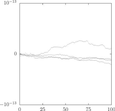
The vector angular momentum is conserved if there are no external torques. The time derivative of the body components of the angular momentum can be written entirely in terms of the body components of the angular momentum, and the three principal moments of inertia. The body components of angular momentum form a self-contained dynamical subsystem.
One choice for generalized coordinates is the Euler angles. They form suitable generalized coordinates, but are otherwise not special or well motivated. The Lagrange equations for the Euler angles are singular for some Euler angles. Other choices of generalized coordinates like the Euler angles have similar problems. Equations of motion using quaternions are nonsingular.
In general the potential energy depends on the details of the mass distribution, and does not separate as the kinetic energy separated into center of mass and relative contributions.
For an axisymmetric top with uniform gravitational acceleration, the potential energy is exactly the potential energy due to elevation of the center of mass. Aspects of the motion of the top are deduced from the conserved quantities. Euler angles are just the right thing for this problem.
For other problems, such as the rotational motion of an out-of-round satellite near a planet, the potential energy cannot be written in finite terms, and judicious approximations must be made. The essential character of such diverse systems as the rotation of the Moon, Hyperion, and Mercury are captured by a simple model problem.
2.14 Projects
Exercise 2.20: Free rigid body
Write and demonstrate a program that reproduces diagrams like figure 2.3 (section 2.8.2). Can you find trajectories that are asymptotic to the unstable relative equilibrium on the intermediate principal axis?
Exercise 2.21: Rotation of Mercury
In the ’60s it was discovered that Mercury has a rotation period that is precisely 2/3 times its orbital period. We can see this resonant behavior in the spin-orbit model problem, and we can also play with nudging Mercury a bit to see how far off the rotation rate can be and still be trapped in this spin-orbit resonance. If the mismatch in angular velocity is too great, Mercury’s rotation is no longer resonantly locked to its orbit. Set ϵ = 0.026 and e = 0.2.
a. Write a program for the spin-orbit problem so this resonance dynamics can be investigated numerically. You will need to know (or, better, show!) that f satisfies the equation
with
Notice that n disappears from the equations if they are written in terms of a new independent variable τ = nt. Also notice that a and R(t) appear only in the combination a/R(t).
b. Show that the 3:2 resonance is stable by numerically integrating the system when the rotation is not exactly in resonance and observing that the angle
c. Find the range of initial
1We put a rubber band or string around the book so that it does not open.
2For an elementary geometric proof see Whittaker [46], p. 2.
3Remember, an orthogonal matrix R satisfies
4The last equality follows from the fact that the rotation of two vectors preserves the dot product:
5We take a 1-by-1 matrix as a number.
6That the inertia tensor transforms in this manner could have been deduced from its definition (2.24). However, it seems that the argument based on the coordinate-system independence of the kinetic energy provides insight.
7If two eigenvalues are not distinct then linear combinations of the associated eigenvectors are eigenvectors. This gives us the freedom to find linear combinations of the eigenvectors that are orthonormal.
8We expect that for each constant of the motion we reduce by one the dimension of the region of the state space explored by a trajectory. This is because a constant of the motion can be used locally to solve for one of the state variables in terms of the others.
9Systems of ODEs that satisfy a Lipschitz condition have unique solutions.
10The deviation of the angular momentum from the principal axis may be due to a number of effects: earthquakes, atmospheric tides, … .
11Here we are using the column-matrix version of the components of the angular momentum, as in equation (2.52).
12Rotating the cross product of two vectors gives the same vector as is obtained by taking the cross product of two rotated vectors:
13In this equation we have a partial derivative with respect to a component of the coordinate argument of the potential energy function. The first subscript on the ∂ symbol indicates the coordinate argument. The second one selects the φ component.
14That the axisymmetric top can be solved in Euler angles is, no doubt, the reason for the traditional choice of the definition of these. For other problems, the Euler angles may offer no particular advantage.
15Here, we do not require that C be larger than A = B, because they are not measured with respect to the center of mass.
16Traditionally, evaluating a definite integral is known as performing a quadrature.
17The Legendre polynomials Pl may be obtained by expanding the expression (1 + y2 − 2yx)−1/2 as a power series in y. The coefficient of yl is Pl(x). The first few Legendre polynomials are: P0(x) = 1, P1(x) = x,
lPl(x) = (2l − 1)xPl−1(x) − (l − 1)Pl−2(x).
18This approximate representation of the potential energy is sometimes called MacCullagh’s formula.
19Traditionally, the point in the orbit at which the two bodies are closest is called the pericenter and the angle f is called the true anomaly.
20The given potential energy differs from the actual potential energy in that non-constant terms that do not depend on θ and consequently do not affect the evolution of θ have been dropped.
21Traditionally, the orbital angular frequency is called the mean motion.
22Deriving the coefficients is a matter of celestial mechanics;
23This method of averaging is rather vague; we will justify it later when we study perturbation theory.
24We could incorporate external torques by using the augmented Euler’s equations (2.83).