6.3  Many Degrees of Freedom

Other problems are encountered in applying perturbation theory to systems with more than a single degree of freedom. Consider a Hamiltonian of the form

where H₀ depends only on the momenta and so is solvable. We assume that the Hamiltonian has no explicit time dependence. We further assume that the coordinates are all angles and that H₁ is a multiply periodic function of the coordinates.

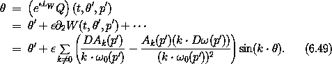
Carrying out a Lie transformation with generator W produces the Hamiltonian

as before. The condition that the order- terms are eliminated is

a linear partial differential equation. By assumption, the Hamiltonian H₀ depends only on the momenta. We define

the tuple of frequencies of the unperturbed system. The condition on W is

As H₁ is a multiply-periodic function of the coordinates, we can write it as a Poisson series:¹

Similarly, we assume W can be written as a Poisson series:

Substituting these into the condition that order- terms are eliminated, we find

The cosines are orthogonal so each term must be individually zero. We deduce

and that the required Lie generator is

There are a couple of problems. First, if A₀ is nonzero then the expression for B₀ involves a division by zero. So the expression for B₀ is not correct. The problem is that the corresponding term in H₁ does not involve . So the integration for B₀ should introduce linear terms in . But this is the same situation that led to the secular terms in the perturbation approximation to the pendulum. Having learned our lesson there, we avoid the secular terms by adjoining this term to the solvable Hamiltonian and excluding k = 0 from the sum for W. We have

and

Another problem is that there are many opportunities for small denominators that would make the perturbation large and therefore not a perturbation. As we saw in the perturbation approximation for the pendulum in terms of the rotor, we must exclude certain regions from the domain of applicability of the perturbation approximation. These excluded regions are associated with commensurabilities among the frequencies ₀(p). Consider the phase-space transformation of the coordinates

So we must exclude from the domain of applicability all regions for which the coefficients are large. If the second term dominates, the excluded regions satisfy

Considering the fact that for any tuple of frequencies ₀(p') we can find a tuple of integers k such that k · (p') is arbitrarily small, this problem of small divisors looks very serious.

However, the problem, though serious, is not as bad as it may appear, for a couple of reasons. First, it may be that A_k ne 0 only for certain k. In this case, only the regions for these terms are excluded from the domain of applicability. Second, for analytic functions the magnitude of A_k decreases strongly with the size of k (see [4]):

for some positive ß and C, and where | k |₊ = | k₀ | + | k₁ | + ··· . At any stage of a perturbation approximation we can limit consideration to just those terms that are larger than a specified magnitude. The size of the excluded region corresponding to a term is of order square root of |A_k(p')| and the inequality (6.51) shows that |A_k(p')| decreases exponentially with the order of the term.

6.3.1  Driven Pendulum as a Perturbed Rotor

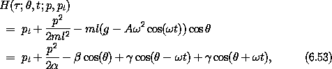
More concretely, consider the periodically driven pendulum. We will develop approximate solutions for the driven pendulum as a perturbed rotor.

We use the Hamiltonian

We can remove the explicit time dependence by going to the extended phase space. The Hamiltonian is

with the constants = ml², ß = mlg, and = (1/2) m l A ² .

With the intent to approximate the driven pendulum as a perturbed rotor, we choose

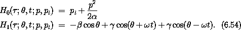
Notice that the perturbation H₁ has only three terms in its Poisson series, so in the first perturbation step only three regions will be excluded from the domain of applicability. The perturbation H₁ is particularly simple: it has only three terms, and the coefficients are constants.

The Lie series generator that eliminates the terms in H₁ to first order in , satisfying

is

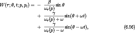
where _r(p) = _2,0 H₀(; , t; p, p_t) = p/ is the unperturbed rotor frequency.

The resulting approximate solution has three regions in which there are small denominators, and so three regions that are excluded from applicability of the perturbative solution. Regions of phase space for which _r(p) is near 0, , and - are excluded. Away from these regions the perturbative solution works well, just as in the rotor approximation for the pendulum. Unfortunately, some of the more interesting regions of the phase space of the driven pendulum are excluded: the region in which we find the remnant of the undriven pendulum is excluded, as are the two resonance regions in which the rotation of the pendulum is synchronous with the drive. We need to develop methods for approximating these regions.