
We can develop an approximation for an isolated resonance region as follows. We again consider Hamiltonians of the form
where H0(t, q, p) =  0(p) depends only on the momenta and so is
solvable. We assume
that the Hamiltonian has no explicit time dependence. We further
assume that the coordinates are all angles, and that H1 is a
multiply periodic function of the coordinates that can be written
0(p) depends only on the momenta and so is
solvable. We assume
that the Hamiltonian has no explicit time dependence. We further
assume that the coordinates are all angles, and that H1 is a
multiply periodic function of the coordinates that can be written

Suppose we are interested in a region of phase space for which n
·  0(p) is near zero, where n is a tuple of integers,
one for each degree of freedom. If we develop the perturbation
theory as before with the generator W that eliminates all terms of
order
0(p) is near zero, where n is a tuple of integers,
one for each degree of freedom. If we develop the perturbation
theory as before with the generator W that eliminates all terms of
order  , then the transformed Hamiltonian is H0, which is
analytically solvable, but there would be terms with n ·
0(p) in the denominator. The resulting solution is not
applicable near this resonance.
, then the transformed Hamiltonian is H0, which is
analytically solvable, but there would be terms with n ·
0(p) in the denominator. The resulting solution is not
applicable near this resonance.
Just as the problem of secular terms was solved by grouping more terms with the solvable part of the Hamiltonian, we can develop approximations that are valid in the resonance region by eliminating fewer terms and grouping more terms in the solvable part.
To develop a perturbative approximation in the resonance region for which n
· 0(p) is near zero, we take the generator W to be

excluding terms in W that lead to small denominators in this region. The transformed Hamiltonian is

where the additional terms are higher-order in . By
excluding the term k = n from the sum in the generating function, that
term is left after the transformation.
The transformed Hamiltonian depends only on a single combination of angles, so a change of variables can be made so that the new transformed Hamiltonian is cyclic in all but one coordinate, which is this combination of angles. This transformed Hamiltonian is solvable (reducible to quadratures).
For example, suppose there are two degrees of freedom  =
(1, 2) and we are interested in a region of phase space
in which n · 0 is near zero, with n = (n1, n2). The
combination of angles n · is slowly varying in the
resonance region. The transformed
Hamiltonian (6.60) is of the
form
=
(1, 2) and we are interested in a region of phase space
in which n · 0 is near zero, with n = (n1, n2). The
combination of angles n · is slowly varying in the
resonance region. The transformed
Hamiltonian (6.60) is of the
form

We can transform variables to  = n1 1 + n2 2,
with second coordinate, say, ' = 2.2
Using the F2-type generating function
= n1 1 + n2 2,
with second coordinate, say, ' = 2.2
Using the F2-type generating function

we find that the transformation is
In these variables the transformed resonance Hamiltonian H'n becomes

This Hamiltonian is cyclic in ', so  ' is constant.
With this constant momentum, the Hamiltonian for the conjugate pair
(,
' is constant.
With this constant momentum, the Hamiltonian for the conjugate pair
(,  ) has one degree of freedom. The solutions are level
curves of the Hamiltonian. These solutions, reexpressed in
terms of the original phase-space coordinates, give the
evolution of H'n.
An approximate solution in the resonance region is therefore
) has one degree of freedom. The solutions are level
curves of the Hamiltonian. These solutions, reexpressed in
terms of the original phase-space coordinates, give the
evolution of H'n.
An approximate solution in the resonance region is therefore

If the resonance regions are sufficiently separated, then a global solution can be constructed by splicing together such solutions for each resonance region.
The resonance Hamiltonian (6.64) has a single degree of freedom and is therefore solvable (reducible to quadratures). We can develop an approximate analytic solution in the vicinity of the resonance by making use of the fact that the solution is valid there. The resonance Hamiltonian can be approximated by a generalized pendulum Hamiltonian.


then the resonance Hamiltonian is

Define the resonance center n by the requirement that the
resonance frequency be zero there:

Now expand both parts of the resonance Hamiltonian about the resonance center:

The first term in the expansion of H''n,0 is a constant and can
be ignored. The coefficient of the second term is zero, from the
definition of n. The third term is the first significant term.
We presume here that the first term of H''n,1 is a nonzero constant.
Now the scale of the separatrix in at resonance is typically
proportional to ()1/2. So the third term of H''n,0
and the first term of H''n,1 are both proportional to .
Subsequent terms are higher-order in . Keeping only the
order- terms, the approximate resonance Hamiltonian is of the form

which is the Hamiltonian for a pendulum with a shifted center in momentum. This is analytically solvable.
Consider the behavior of the periodically driven
pendulum in the vicinity of the resonance r(p) = .
The Hamiltonian (6.54) for the driven
pendulum has three resonance terms in H1. The full
generator (6.56) has three terms that are
designed to eliminate the corresponding resonance terms in the
Hamiltonian. The resulting approximate solution has small
denominators close to each of the three resonances,
r(p) = 0, r(p) = , and
r(p) = - .
To develop a resonance approximation near r(p) = , we
do not include the corresponding term in the generator, so that the
corresponding term is left in the Hamiltonian. It is helpful to give names to the
various terms in the full generator (6.56):
The full generator is W0 + W- + W+.
To investigate the motion in the phase space near the resonance
r(p) = (the "+" resonance), we use the generator that
excludes the corresponding term

With this generator the transformed Hamiltonian is

After we exclude the higher-order terms, this Hamiltonian has only a single combination of coordinates, and so can be transformed into a Hamiltonian that is cyclic in all but one degree of freedom. Define the transformation through the mixed-variable generating function

Expressed in these new coordinates, the resonance Hamiltonian is
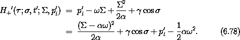
This Hamiltonian is cyclic in t', so the solutions are level curves
of H+' in (, ). Actually, more can be said here
because H+' is already of the form of a pendulum shifted in the
direction by  and shifted by
  in phase. The
shift by comes about because the sign of the cosine term is
positive, rather than negative as in the usual pendulum. A sketch of
the level curves is given in figure 6.8.
in phase. The
shift by comes about because the sign of the cosine term is
positive, rather than negative as in the usual pendulum. A sketch of
the level curves is given in figure 6.8.
Exercise 6.2. Resonance width
Verify that the half-width of the resonance region is 2 (
 )1/2.
)1/2.
Exercise 6.3. With the computer
Verify, with the computer, that with the generator W+ the
transformed Hamiltonian is given by equation (6.75).
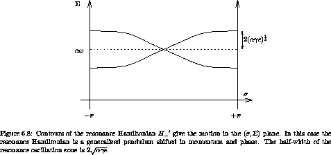
An approximate solution of the driven pendulum near the r(p) =
resonance is

To find out to what extent the approximate solution models the actual
driven pendulum, we make a surface of section using this approximate
solution and compare it to a surface of section for the actual driven
pendulum. The surface of section for the approximate solution in the
resonance region is shown in figure 6.9. A
surface of section for the actual driven pendulum is shown in the lower part of
figure 6.10. The correspondence is surprisingly
good.
Note how the resonance island is not symmetrical about a
line of constant momentum. The resonance Hamiltonian is symmetrical
about = , and by itself would give a
symmetric resonance island (see figure 6.8). The necessary distortion is introduced by
the W+ transformation that eliminates the other resonances.
Indeed, in the full section the distortion appears to be generated by
the nearby r(p) = 0 resonance ``pushing away'' nearby
features so that it has room to fit.
However, some features of the actual section are not represented;
for instance, there is a small chaotic zone near the actual
separatrix.
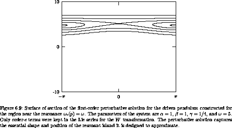
The perturbation solution near the r(p) = 0 resonance merges
smoothly with the perturbation solutions for the r(p) =
and r(p) = - resonances. We can make a
composite perturbative solution by using the appropriate resonance
solution for each region of phase space. A surface of section for the
composite perturbative solution is shown in the upper part of
figure 6.10, as is
the corresponding surface of section for the actual driven pendulum.
The perturbative solution
captures many features seen on the actual section.
However, the first-order perturbative solution does not capture the
resonant islands between the two primary resonances or the secondary
island chains contained within a primary resonance region. Also, the
first-order perturbative solution does not show the chaotic zone near
the separatrix apparent in the surface of section for the actual
driven pendulum.
We see, from the comparisons of the sections of the first-order perturbative solutions for the various resonance regions, that the section for the actual driven pendulum can be approximately constructed by combining the approximations developed for each resonance. The shapes of the resonance regions are distorted by the transformations that eliminate the nearby resonances, so the resulting pieces fit together consistently. The predicted width of each resonance region agrees with the actual width: it is not substantially changed by the distortion of the region introduced by the elimination of the other resonance terms. Not all the features of the actual section are reproduced in this composite of first-order approximations: there are chaotic zones and islands that do not appear in this collage of first-order approximations.
For larger drives, the approximations derived by first-order perturbations are worse. In the lower part of figure 6.11, with drive larger by a factor of five we lose the invariant curves that separate the resonance regions. The main resonance islands persist, but the chaotic zones near the separatrices have merged into one large chaotic sea.
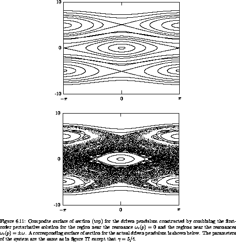
The composite first-order perturbative solution for the more strongly driven
pendulum in the upper part of figure 6.11 still approximates the
centers of the main resonance islands reasonably well, but it fails as
we move out and encounter the secondary islands that are visible in
the resonance region for r(p) = . Here the
approximations for the two regions do not fit together so well. The
chaotic sea is found in the region where the perturbative solutions do
not match.
The locations and widths of the primary resonance islands can often be
read straight off the Hamiltonian when expressed as a Poisson series.
For each term in the series for the perturbation there is a
corresponding resonance island. The width of the island can often be
simply computed from the coefficients in the Hamiltonian. So just by
looking at the Hamiltonian we can get a good idea of what sort of
behavior we will see on the surface of section. For instance, in
the driven pendulum, the
Hamiltonian (6.53) has three
terms. We could anticipate, just from looking at the Hamiltonian,
that three main resonance islands are to be found on the surface
of section. We know that these islands will be located where the
resonant combination of angles is slow. So for the periodically
driven pendulum the resonances occur near r(p) = ,
r(p) = 0, and r(p) = - . The approximate widths
of the resonance islands can be computed with a simple calculation.
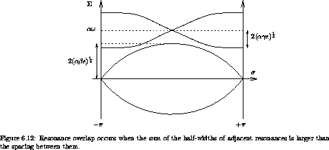
As the size of the drive increases, the chaotic zones near the
separatrices get larger and then merge into a large chaotic sea. The
resonance-overlap criterion gives an analytic estimate of when this
occurs. The basic idea is to compare the sum of the widths of
neighboring resonances with their separation. If the sum of the
half-widths is greater than the separation, then the resonance-overlap
criterion predicts there will be large-scale chaotic behavior near the
overlapping resonances. In the case of the periodically driven
pendulum, the half-width of the r(p) = 0 resonance is
2 ( ß)1/2 and the half-width of the
r(p) = resonance is 2 ( )1/2 (see
figure 6.12). The
separation of the resonances is . So resonance overlap
occurs if

The amplitude of the drive enters through . Solving, we
find the value of above which resonance overlap occurs.
For the parameters = ß = 1, = 5 used in
figures 6.9-6.11,
the resonance overlap value of is 9/4. We see that,
in fact, the chaotic zones have already merged for = 5/4. So
in this case the resonance-overlap criterion overestimates the
strength of the resonances required to get large-scale
chaotic behavior. This is typical of the resonance-overlap criterion.
A way of thinking about why the resonance-overlap criterion usually overestimates the strength required to get large-scale chaos is that other effects must be taken into account. For instance, as the drive is increased second-order resonances appear between the primary resonances; these resonances take up space and so resonance overlap occurs for smaller drive than would be expected by considering the primary resonances alone. Also, the chaotic zones at each separatrix have area that must be accounted for.
As the drive is increased, a variety of new islands emerge, which are not evident in the original Hamiltonian. To find approximations for motion in these regions we can use higher-order perturbation theory. The basic plan is the same as before. At any stage the Hamiltonian (which is perhaps a result of earlier stages of perturbation theory) is expressed as a Poisson series (a multiple-angle Fourier series). The terms that are not resonant in a region of interest are eliminated by a Lie transformation. The remaining resonance terms involve only a single combination of angle and are thus solvable by making a canonical transformation to resonance coordinates. We complete the solution and transform back to the original coordinates.
Let's find a perturbative approximation for the second-order islands
visible in figure 6.10 between the r(p) =
0 resonance and the r(p) = - resonance. The details
are messy, so we will just give a few intermediate results.
This resonance is not near the three primary resonances, so we can use the full generator (6.56) to eliminate those three primary resonance terms from the Hamiltonian. After this perturbation step the Hamiltonian is too hairy to look at.
We expand the transformed Hamiltonian in Poisson form and divide the terms into those that are resonant and those that are not. The terms that are not resonant can be eliminated by a Lie transform. This Lie transform leaves the resonant terms in the Hamiltonian and introduces an additional distortion to the curves on the surface of section. In this case this latter distortion is small, but very messy to compute, so we will just not include this effect. The resonance Hamiltonian is then (after considerable algebra)
This is solvable because there is only a single combination of coordinates.
We can get an analytic solution by making the pendulum
approximation. The Hamiltonian is already quadratic in the momentum
p, so all we need to do is evaluate the coefficient of the potential
terms at the resonance center p2:1 = / 2. The
resonance Hamiltonian, in the pendulum approximation, is

Carrying out the transformation to the resonance variable = 2
- t reduces this to a pendulum Hamiltonian with a
single degree of freedom. Combining the analytic solution of this
pendulum Hamiltonian with the transformations generated by the full
W, we get an approximate perturbative solution

A surface of section in the appropriate resonance region using this solution is shown in figure 6.13. Comparing this to the actual surface of section (figure 6.10), we see that the approximate solution provides a good representation of this resonance motion.

As a second application, we use second-order perturbation theory to investigate the inverted vertical equilibrium of the periodically driven pendulum.
Here, the procedure parallels that just followed, but we focus
on a different set of resonance terms. The terms that are slowly
varying for the vertical equilibrium are those that involve
but do not involve t, such as cos () and cos (2 ).
So we want to use the generator W+ + W- that eliminates the
nonresonant terms involving combinations of and t,
while leaving the central resonance. After the Lie transform of the
Hamiltonian with this generator, we write the transformed Hamiltonian
as a Poisson series and collect the resonant terms. The transformed
resonance Hamiltonian is

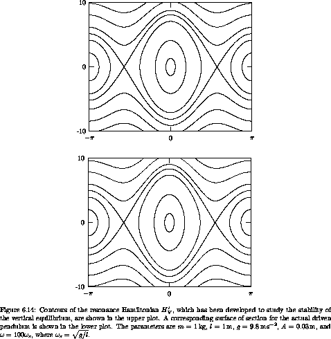
Figure 6.14 shows contours of this resonance Hamiltonian H'V and a surface of section for the actual driven pendulum for the same parameters. The behavior of the resonance Hamiltonian is indistinguishable from that of the actual driven pendulum. The theory does especially well here; there are no nearby resonances because the drive frequency is high.
We can get an analytic estimate for the stability of the inverted
vertical equilibrium by carrying out a linear stability analysis of
the resonance Hamiltonian of the fixed point = , p = 0. The
algebra is somewhat simpler if we first make the pendulum
approximation about the resonance center. The resonance Hamiltonian
is then approximately

Linear stability analysis of the inverted vertical equilibrium indicates stability for

In terms of the original physical parameters, the vertical equilibrium is linearly stable if

where s = (g/l)1/2, the small-amplitude oscillation frequency. For the vertical equilibrium to be
stable, the scaled product of the amplitude of the drive and the drive
frequency must be sufficiently large.
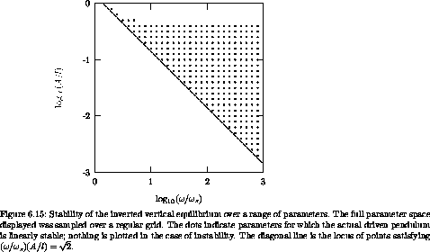
This analytic estimate is compared with the behavior of the driven
pendulum in figure 6.15. For any given
assignment of the parameters, the driven pendulum can be tested for the
linear stability of the inverted vertical equilibrium by the methods
of chapter 4; this
involves determining the roots of the characteristic polynomial for a
reference orbit at the resonance center. In the figure the stability
of the inverted vertical equilibrium was assessed at each point of a
grid of assignments of the parameters. A dot is shown for
combinations of parameters that are linearly stable. The
diagonal line is the analytic boundary of the region of stability of
the inverted equilibrium: (/s)(A/l) = (2)1/2. We see
that the boundary of the region of stability is well approximated by
the analytic estimate derived from perturbation theory. Note that
for very high drive amplitudes there is another region of instability,
which is not captured by this perturbation analysis.
2 Any linearly independent combination will be acceptable here.