For the driven pendulum we observe that as the amplitude of the drive is increased the separatrix of the undriven pendulum is where the most prominent chaotic zone appears. Here we examine in great detail the motion in the vicinity of the separatrix. What emerges is a remarkably complicated picture, first discovered by Henri Poincaré. Indeed, Poincaré stated (see the epigraph to this chapter) that the picture that emerged was so complicated that he was not even going to attempt to draw it. We will review the argument leading to the picture, and compute enough of it to convince ourselves of its reality.
The separatrix of the undriven pendulum is made up of two trajectories that are asymptotic to the unstable equilibrium. In the driven pendulum with zero drive, an infinite number of distinct orbits lie on the separatrix; they are distinguished by the phase of the drive. These orbits are asymptotic to the unstable fixed point both forward and backward in time.

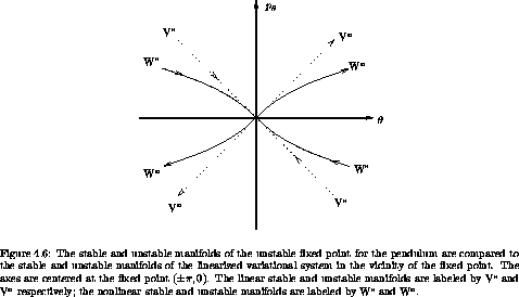
Notice that close to the unstable fixed point the sets of points that are asymptotic to the unstable equilibrium must be tangent to the linear variational eigenvectors at the fixed point. (See figure 4.6.) In a sense, the sets of orbits that are asymptotic to the fixed point are extensions to the nonlinear problem of the sets of orbits that are asymptotic to the fixed point in the linearized problem.
The set of points that are asymptotic to an unstable fixed point forward in time is called the stable manifold of the fixed point. The set of points that are asymptotic to an unstable fixed point backward in time is called the unstable manifold. For the driven pendulum with zero-amplitude drive, all points on the separatrix are asymptotic both forward and backward in time to the unstable fixed point. So in this case the stable and unstable manifolds coincide.
If the drive amplitude is nonzero then there are still one-dimensional sets of points that are asymptotic to the unstable fixed point forward and backward in time: there are still stable and unstable manifolds. Why? The behavior near the fixed point is described by the linearized variational system. For the linear variational system, points in the space spanned by the unstable eigenvector, when mapped backwards in time, are asymptotic to the fixed point. Points slightly off this curve may initially approach the unstable equilibrium, but eventually will fall away to one side or the other. For the driven system with small drive, there must still be a curve that separates the points that fall away to one side from the points that fall away to the other side. Points on the dividing curve must be asymptotic to the unstable equilibrium. The dividing set cannot have positive area because the map is area preserving.
For the zero-amplitude drive case, the stable and unstable manifolds are contours of the conserved Hamiltonian. For nonzero amplitude the Hamiltonian is no longer conserved, and the stable manifolds and unstable manifolds no longer coincide. This is generally true for non-integrable systems: stable and unstable manifolds do not coincide.
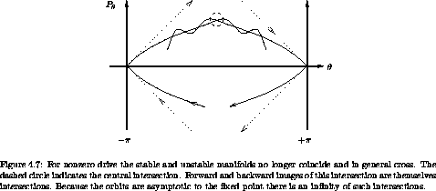
If the stable and unstable manifolds no longer coincide, where do they go? In general, the stable and unstable manifolds must cross one another. The only other possibilities are that they run off to infinity or spiral around. Area preservation can be used to exclude the spiraling case. We will see that in general there are barriers to running away. So the only possibility is that the stable and unstable manifolds cross, as is illustrated in figure 4.7. The point of crossing of a stable and unstable manifold is called a homoclinic intersection if the stable and unstable manifolds belong to the same unstable fixed point. It is called a heteroclinic intersection if the stable and unstable manifolds belong to different fixed points.
If the stable and unstable manifolds cross once then there are an infinite number of other crossings. The intersection point belongs to both the stable and unstable manifolds. That it is on the unstable manifold means that all images forward and backward in time also belong to the unstable manifold, and likewise for points on the stable manifold. Thus all images of the intersection belong to both the stable and unstable manifolds. So these images must be additional crossings of the two manifolds.
We can deduce that there are still more intersections of the stable and unstable manifolds. The maps we are considering not only preserve area but also orientation. In the proof of Liouville's theorem we showed that the determinant of the transformation is one, not just magnitude one. If we consider little segments of the stable and unstable manifolds near the intersection point, then these segments must map near the image of the intersection point. That the map preserves orientation implies that the manifolds are crossing one another in the same sense as at the previous intersection. Therefore there must have been at least one more crossing of the stable and unstable manifolds in between these two. This is illustrated in figure 4.8. Of course, all forward and backward images of these intermediate intersections are also intersections.
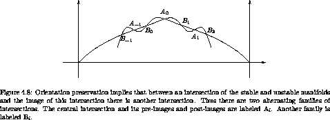
As the picture gets more complicated, keep in mind that the stable manifold cannot cross itself and the unstable manifold cannot cross itself. Suppose one did, say by making a little loop. The image of this loop under the map must also be a loop. So if there were a loop there would have to be an infinite number of loops. That would be okay, but what happens as the loop gets close to the fixed point? There would still have to be loops, but then the stable and unstable manifolds would not have the right behavior: the stable and unstable manifolds of the linearized map do not have loops. Therefore, the stable and unstable manifolds cannot cross themselves.7
We are not done yet! The lobes that are defined by successive crossings of the stable and unstable manifolds enclose a certain area. The map is area preserving so all images of these lobes must have the same area. As the lobes approach the fixed point, we get an infinite number of lobes with a base of exponentially shrinking length. The stable and unstable manifolds cannot cross themselves, so to pack these lobes together on the plane the lobes must stretch out to preserve area. We see that the length of the lobe must grow roughly exponentially (it may not be uniform in width so it need not be exactly exponential). This exponential lengthening of the lobes no doubt bears some responsibility for the exponential divergence of nearby trajectories of chaotic orbits, but does not prove it. It does, however, suggest a connection between the fact that chaotic orbits appear to occupy an area on the section and the fact that nearby chaotic orbits diverge exponentially.
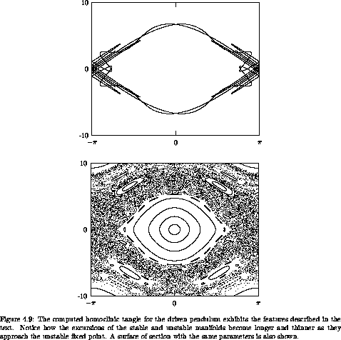
Actually, the situation is even more complicated. As the lobes stretch, they form tendrils that wrap around the separatrix region. The tendrils of the unstable manifold can cross the tendrils of the stable manifold. Each point of crossing is a new homoclinic intersection, and so each pre- and post-image of this point belongs to both the stable and unstable manifolds, indicating another crossing of these curves. We could go on and on. No wonder Poincaré refused to draw this mess.
Exercise 4.5. Homoclinic paradox
How do we fit an infinite number of copies of a finite area in a finite region, without allowing the stable and unstable manifolds to cross themselves? Resolve this apparent paradox.
The homoclinic tangle is not just a bad dream. We can actually compute it.
Very close to an unstable fixed point the stable and unstable manifolds become indistinguishable from the rays along the eigenvectors of the linearized system. So one way to compute the unstable manifold is to take a line of initial conditions close to the fixed point along the unstable manifold of the linearized system and evolve them forward in time. Similarly, the stable manifold can be constructed by taking a line of initial conditions along the stable manifold of the linearized system and evolving them backward in time.
We can do better than this by choosing some parameter (like arc length) along the manifold and for each parameter deciding how many iterations of the map would be required to take the point back to within some small region of the fixed point. We then choose an initial condition along the linearized eigenvectors and iterate the point back with the map. This idea is implemented in the following program:
(define ((unstable-manifold T xe ye dx dy rho eps) param)
(let ((n (floor->exact (/ (log (/ param eps)) (log rho)))))
((iterated-map T n) (+ xe (* dx (/ param (expt rho n))))
(+ ye (* dy (/ param (expt rho n))))
cons
(lambda () (error "Failed")))))
where T is the map, xe and ye are the coordinates of the fixed point, dx and dy are components of the linearized eigenvector, rho is the characteristic multiplier, eps is a scale within which the linearized map is a good enough approximation to T, and param is a continuous parameter along the manifold. The program assumes that there is a basic exponential divergence along the manifold -- that is why we take the logarithm of param to get initial conditions in the linear regime. This assumption is not exactly true, but it is good enough for now.
The curve is generated by a call to plot-parametric-fill, which recursively subdivides intervals of the parameter until there are enough points to get a smooth curve.
(define (plot-parametric-fill win f a b near?)
(let loop ((a a) (xa (f a)) (b b) (xb (f b)))
(if (not (close-enuf? a b (* 10 *machine-epsilon*)))
(let ((m (/ (+ a b) 2)))
(let ((xm (f m)))
(plot-point win (car xm) (cdr xm))
(if (not (near? xa xm))
(loop a xa m xm))
(if (not (near? xb xm))
(loop m xm b xb)))))))
The near? argument is a test for whether two points are within a given distance of each other in the graph. Because some coordinates are angle variables, this may involve a principal value comparison. For example, for the driven pendulum section, the horizontal axis is an angle but the vertical axis is not, so the picture is on a cylinder:
(define (cylinder-near? eps)
(let ((eps2 (square eps)))
(lambda (x y)
(< (+ (square ((principal-value pi)
(- (car x) (car y))))
(square (- (cdr x) (cdr y))))
eps2))))
Figure 4.9 shows a computation of the homoclinic
tangle for the driven pendulum. The parameters are m = 1 kg,
g = 9.8 m s-2, l = 1 m,  = 4.2(g/l)1/2, and
amplitude A = 0.05 m. For reference,
figure 4.9 shows a surface of section for
these parameters on the same scale.
Exercise 4.6. Computing homoclinic tangles
a. Compute stable and unstable manifolds for the standard map.
b. Identify the features on the homoclinic tangle that entered the argument about its existence, such as the central crossing of the stable and unstable manifolds, etc.
c. Investigate the errors in the process. Are the computed manifolds really correct or a figment of wishful thinking? One could imagine that the errors are exponential and the computed manifolds have nothing to do with the actual manifolds.
d. How much actual space is taken up by the homoclinic tangle? Consider a value of the coupling constant K = 0.8. Does the homoclinic tangle actually fill out the apparent chaotic zone?
7 Sometimes it is argued that the stable and unstable manifolds cannot cross themselves on the basis of the uniqueness of solutions of differential equations. This argument is incorrect. The stable and unstable manifolds are not themselves solutions of a differential equation, they are sets of points whose solutions are asymptotic to the unstable fixed points.