3.3  One Degree of Freedom

The solutions of time-independent systems with one degree of freedom can be found by quadrature. Such systems conserve the Hamiltonian: the Hamiltonian has a constant value on each realizable trajectory. We can use this constraint to eliminate the momentum in favor of the coordinate. Thus Hamilton's equations reduce to a single equation Dq(t) = f(q(t)). The solution q can be expressed as a definite integral.

A geometric view reveals more structure. Time-independent systems with one degree of freedom have a two-dimensional phase space. Energy is conserved, so all orbits are level curves of the Hamiltonian. The possible orbit types are restricted to curves that are contours of a real-valued function. The possible orbits are paths of constant altitude in the mountain range on the phase plane described by the Hamiltonian.

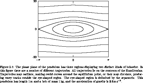
Only a few characteristic features are possible. There are points that are stable equilibria of the dynamical system. These are the peaks and pits of the Hamiltonian mountain range. These equilibria are stable in the sense that neighboring trajectories on nearby contours stay close to the equilibrium point. There are orbits that trace simple closed curves on contours that surround a peak or pit, or perhaps several peaks. There are also trajectories lying on contours that cross at a saddle point. The crossing point is an unstable equilibrium, unstable in the sense that neighboring trajectories leave the vicinity of the equilibrium point. Such contours that cross at saddle points are called separatrices (singular: separatrix), contours that ``separate'' two regions of distinct behavior.

At every point Hamilton's equations give a unique rate of evolution and direct the system to move perpendicular to the gradient of the Hamiltonian. At the peaks, pits, and saddle points, the gradient of the Hamiltonian is zero, so according to Hamilton's equations these are equilibria. At other points, the gradient of the Hamiltonian is nonzero, so according to Hamilton's equations the rate of evolution is nonzero. Trajectories evolve along the contours of the Hamiltonian. Trajectories on simple closed contours periodically trace the contour. At a saddle point, contours cross. The gradient of the Hamiltonian is zero at the saddle point, so a system started at the saddle point does not leave the saddle point. On the separatrix away from the saddle point the gradient of the Hamiltonian is not zero, so trajectories evolve along the contour. Trajectories on the separatrix are asymptotic forward or backward in time to a saddle point. Going forward or backward in time, such trajectories forever approach an unstable equilibrium but never reach it. If the phase space is bounded, asymptotic trajectories that lie on contours of a smooth Hamiltonian are always asymptotic to unstable equilibria at both ends (but they may be different equilibria).

These orbit types are all illustrated by the prototypical phase plane of the pendulum (see figure 3.4). The solutions lie on contours of the Hamiltonian. There are three regions of the phase plane; in each the motion is qualitatively different. In the central region the pendulum oscillates; above this there is a region in which the pendulum circulates in one direction; below the oscillation region the pendulum circulates in the other direction. In the center of the oscillation region there is a stable equilibrium, at which the pendulum is hanging motionless. At the boundaries between these regions, the pendulum is asymptotic to the unstable equilibrium, at which the pendulum is standing upright.¹⁸ There are two asymptotic trajectories, corresponding to the two ways the equilibrium can be approached. Each of these is also asymptotic to the unstable equilibrium going backward in time.